Cellular Textures

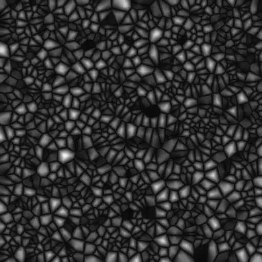
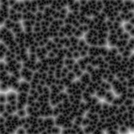
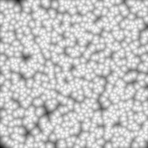
The article “Making Cellular Textures” gives a good description of how you would go about generating textured images like the ones shown below.

The authors’ descriptions and pseudocode provide the basis for the implementation of a CLI texture generator. This article describes such a tool and its performance when generating a number of different textures.

Texture Parameters

The goal of the tool is to generate a texture as a MxN grayscale PNG. The program exposes five key parameters that control the look of the output image:

The Algorithm

The process for generating a texture is as follows:

• Create a MxN grid of pixels.
• Generate --num-points random texture points. All points must lie within the bounds of the pixel grid.
• For each pixel:
  • Find the --num-neighbors nearest texture points.
  • Calculate the distance from the pixel to each neighboring texture point. If tiling is active, apply a modified distance formula that accounts for wrapping around the edges of the pixel grid.
  • Apply the --dist-op operation to the collection of distances. For example, if in the previous step you computed the distances 1, 2, 3, and your --dist-op was multiplication, you would compute \(dist = 1 * 2 * 3 = 6\).
  • Cache each pixel’s \(dist\) value.
  • Keep track of the minimum and maximum \(dist\) values: \(mindist\) and \(maxdist\).
• Iterate over all pixels once again. For each pixel:
  • Compute the grayscale value of the ith pixel, \(c_i\):

\[c_i = \frac{(dist_i - mindist)}{(maxdist - mindist)} * 255\]

• Write the pixels to a grayscale PNG output file.

The Layman’s Explanation

The formulas and numbers can get confusing. The core idea is that you are iterating a grid of grayscale pixels. You want to determine how light or dark each pixel should be. You generate a set of random “texture points” within the bounds of the image. Then you find the \(k\) nearest texture points of each pixel and apply an arbitrary formula to the collection of distances from each of the \(k\) neighbors to the pixel. Applying the formula generates a single “distance” value. You later use this distance value along with the global max and min distances to determine the color of the pixel.

The number of neighbors and the operation you apply creates drastic changes in the output. For example, set --num-neighbors to 2 and --dist-op to minus and you get the following scaly image:

Set --num-neighbors to 1 and --dist-op to multiply and you get the following dotted texture:

The CLI tool is interesting because you can write a script to tweak the parameters generating numerous textures. The video that follows shows some interesting textures generated by running a simple bash script:

#!/bin/bash

for i in $(seq 0 9);
do
    ./ctext 512 512 "sub_1000_$i.png" -k "$i" -d "-"
done

Finding Nearest Neighbors

Given a big enough image and enough texture points, texture generation can be a slow process. You spend the majority of the time computing the distance to the nearest neighbors of each pixel as shown in the KCachegrind capture below:

The capture shows a single ctext run:

ctext 128 128 test.png --num-neighbors 1 --dist-op "-"

The run uses a brute force, \(\mathcal{O}(n^2)\) algorithm, where \(n\) is the number of texture points.

The “Making Cellular Textures” article suggests a number of tree data structures that could help speed up the search. Among these is the K-D Tree. There are a few C++ K-D Tree implementations floating around online. This C++ implementation for nearest neighbor and k nearest neighbors is one of the better options given it comes with solid unit/benchmark tests.

You’d think a \(\mathcal{O}(logn)\) nearest neighbor search complexity would grant a massive speedup. Measurements showed otherwise:

The graph shows the performance of the brute force algorithm versus a 2-D tree on the command

ctext 1024 1024 --num-neighbors=1 --dist-op="-" --num-points=<VARIABLE>

The tree performs about the same or worse in some instances. Why? It’s likely because there’s a significant cost to constructing the tree. The worst case complexity for constructing the tree is \(\mathcal{O}(nlog^2n)\). Then add in that the search complexity is on average \(\mathcal{O}(logn)\). The distribution of the random points also plays a key role. The more uniformly distributed the points are, the more balanced the tree will be. Some of those large spikes to the right might be the result of searches on a “skewed” tree.

Conclusion

With some basic math and computer science, you can write a CLI tool to help you explore the “cellular texture space.” The end result: some neat looking pictures.

The complete project source is available on GitHub under cellular_textures. Note, this project has since been rewritten in Rust. The Rust version of the program uses a K-D tree for nearest neighbor searches exclusively. The performance of the Rust implementation is comparable to that of the original C++ implementation.