This guide will walk you through a “hack” for setting up the Pi-hole on a network that uses an Xfinity modem/router.

Getting the Pi-hole to work with Xfinity hardware can be tricky for two reasons:

• Xfinity blocks you from changing the DNS settings of the device.
• Xfinity blocks you disabling the DHCP server function which blocks you from using the official workaround described here.

With neither of those options available, your fallback is to set the Pi-hole as the DNS server for each individual device on your network. However, this isn’t always possible. For example, if you have a Roku Smart TV, Roku blocks you from changing the DNS settings on the device too!

You’d think you’re shit out of luck at this point and have to dump some money on a new modem/router (not a terrible idea but costly). There is an alternative solution.

The Hack

The executive summary:

• Narrow the range of DHCP addresses served by the Xfinity DHCP server to a single address.
• Reserve that single address for the Pi-hole.
• Enable the DHCP server function of the Pi-hole.

Any new device that connects to the network gets an IP address from the Pi-hole DHCP server. All that device’s DNS request will get routed through the Pi-hole as desired. You don’t have to touch any additional settings on the Xfinity device nor any of the devices on your network!

Preparing the Pi-hole

This article assumes you have already installed the Pi-hole on a Raspberry Pi or other supported device. Further, you followed the warning on installation that has you set a static IP on the device.

To make life easier in the following steps, connect a keyboard, monitor, and mouse to the Pi-hole.

Enabling Configuration of Your Xfinity Modem/Router

To get started configuring your device, you’ll need access to both the Xfinity app and the admin web portal.

You can download the Xfinity app from the Google Play Store or Apple App Store. Once you have the app installed, scan the QR code on the bottom of the device to register it. Under your WiFi device, go to “Advanced Settings -> Gateway admin tool” and enable the admin web portal.

From a web browser on the Pi-hole device, navigate to https://10.0.0.1 and log in with the credentials you set up in the Xfinity app. Navigate using the menu on the left to “Gateway -> Connection -> Local IP Network.” You should see your Xfinity device’s DHCP settings as shown below.

DHCP Setup

Follow these steps to configure DHCP both on the Xfinity device and the Pi-hole.

1. Disconnect all devices from the network except the Pi-hole device.

2. If you have port forwarding rules, jot down the rules and remove them. You can find the rules in the Xfinity app under “Advanced Settings -> Port forwarding.”

   

3. From the Xfinity app, select each “Disconnected Device” individually and select “Forget Device.” Note, that you might have to wait ~10 minutes for the device to show up in the app as a “Disconnected Device.” If you’re impatient, you can disconnect all devices and just reboot the gateway.

   

4. From the Xfinity admin portal, navigate to “Gateway -> Connected Devices.” Select the Pi-hole device and select “Reserve IP Address.”

   

5. From the Xfinity admin web portal, navigate to “Gateway -> Connection -> Local IP Network.” Change the “DHCP Start” and “DHCP End” addresses to a range that includes your Pi-hole’s static IP address. For example, if your Pi-hole has address 10.0.0.247, then you could set the “DHCP Start” to 10.0.0.246 and the “DHCP End” to 10.0.0.247. If you had port forwarding rules, make sure the range of addresses includes one IP per machine that had a port forwarding rule.

6. From the Pi-hole admin web portal, navigate to “Settings -> DHCP.” Enable the DHCP server and set the range of addresses. Make sure that the range does not overlap with the Xfinity DHCP range.

   

7. Reboot the Pi-hole device.

At this point, viewing the “Connected Devices” page of the Xfinity app, you should only see the Pi-hole device connected.

Reconnecting Devices

You’re now going to start reconnecting devices to the network. There’s two paths here: with port forwarding rules and without port forwarding rules.

With Port Forwarding Rules

1. Reconnect each machine that had a rule first.
2. Reconfigure each port forwarding rule using the Xfinity app.
3. Connect all other devices to the network.

Without Port Forwarding Rules

1. First, connect a device for which you can configure the DNS settings directly. For example, a Windows, Linux, or Mac desktop.
2. From the Xfinity admin web portal, navigate to “Gateway -> Connections” and select the device you just connected. Select “Reserve IP Address.”
3. Configure the device to use the Pi-hole as its DNS server.
4. Connect all other devices to the network. No need to configure the DNS settings on any of these devices.

(1) is necessary because the DHCP start and end addresses can’t be the same. The Xfinity device therefore will always assign the second IP address in the range to the first device that connects to the network. As long as that device has configurable DNS, you can set it’s DNS to the Pi-hole and set its IP to reserved. That ensures that address is always filled by a device that uses the Pi-hole for DNS. All other devices will get an IP from the Pi-hole DHCP server and will automatically use the Pi-hole for DNS (even consumer-unfriendly Roku devices).

This is a short guide walking you through the process of setting up the DreamBot Old School RuneScape Botting Client on a Raspberry Pi. While this guide uses a Raspberry Pi Model 3 B+, the steps are near identical on later models of the Pi. Note, that you’ll want a Raspberry Pi 4 or later with at least 2GB of RAM to run DreamBot with reasonable performance.

1. Download and flash the latest Raspberry Pi OS image to a microSD card. You can use Raspberry Pi Imager to simplify this process. Here’s a video showing how to do this:

2. Login to your Raspberry Pi and open a terminal.

3. Update the system and install the latest Java Runtime Environment:

   sudo apt update && sudo apt upgrade -y
   sudo apt install default-jre -y

4. Download the latest DreamBot client JAR file:

   curl https://downloads.dreambot.org/launcher/Launcher.jar -o Launcher.jar

5. Run the DreamBot client:

   java -jar Launcher.jar

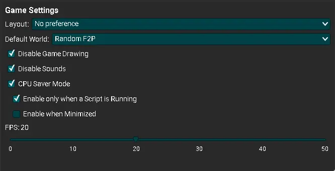
Optionally, you can adjust a couple of DreamBot client settings to improve performance. The recommended Game Settings to adjust are:

• CPU Saver: Check this box and the “Enable only when Script is Running” sub-option.
• Adjust the FPS: Move the slider left or right to decrease/increase FPS. A lower FPS will reduce CPU usage.
• Disable Game Drawing: Check this box to disable game drawing. This will make it so you can’t see what the bot is doing so only use this option with reliable scripts!

Here’s a screen cap of the recommended settings:

This article explains how to configure CopilotChat to use a custom provider. CopilotChat is a NeoVim plugin that provides a LLM chat interface and real-time suggestions. Typically, you use CopilotChat with GitHub Copilot. However, it also supports custom providers. This is especially useful if you work a job where they forbid GitHub Copilot but provide internal LLM services.

Lazy Configuration

It’s assumed you’re using NeoVim with the Lazy plugin manager. Below is the Lazy configuration for CopilotChat with a custom provider.

{
  "CopilotC-Nvim/CopilotChat.nvim",
  branch = "main",
  event = "VeryLazy",
  dependencies = {
    { "github/copilot.vim" },
    { "nvim-lua/plenary.nvim" },
  },
  opts = {
    model = "gemma-4-31b-it", -- Update this to match the id of a provider model
    providers = {
      <COMPANY_NAME> = {
        get_url = function()
          return "<API_BASE_URL>/v1/chat/completions"
        end,
        get_headers = function()
          return {
            ["Authorization"] = "Bearer <YOUR_API_KEY>",
          }
        end,
        get_models = function()
          return { { id = "gemma-4-31b-it", name = "Gemma 4-31B-it" } }
        end,
        prepare_input = function(data, dev)
          return require("CopilotChat.config.providers").copilot.prepare_input(data, dev)
        end,
        prepare_output = function(data, dev)
          return require("CopilotChat.config.providers").copilot.prepare_output(data, dev)
        end,
      },
    },
  }
}

There’s a couple fields that require adjustment on your end marked with <...> in the configuration:

• COMPANY_NAME: This is the name of your provider. You can choose any name you want, but it should be unique and descriptive.
• API_BASE_URL: This is the base address for your provider’s API. You’ll have to consult your provider’s docs to find out what this is.
• YOUR_API_KEY: This is the API key for your provider. Again, consult your provider’s docs to find out how to generate a user API key or a get an organization key.

The get_models() function is also of interest. Most providers have a catalog of LLMs that you can use. In the example, a single model called gemma-4-31b-it gets referenced. You can add as many models as you want from your provider’s catalog. Just make sure the id field matches the model name as defined by your provider.

Save and reload your configuration. If all goes well, you should see your providers’ models in the :CopilotChatModels menu.

Worth mentioning, there are more functions you can override in the provider interface provided by CopilotChat. For the full listing see Providers.

This is a 2026 follow on to Setting Up a Local LLM. This article will discuss running two local models using llama.cpp. One model will be a beefier chat model capable of handling more complex tasks. The second model will be a smaller model, tuned for auto completion and basic code generation. You’ll see how to integrate both into your NeoVim workflow using the CodeCompanion and llama.vim plugins.

Installing llama.cpp

llama.cpp is a collection of tools for running open models on your hardware. You can install the tools in a variety of ways. In this guide, you’ll compile it from source. Why? Compiling from source creates binaries optimized to your specific hardware. This may or may not lead to noticeable performance gains. That said, it’s easy to do, ensures you have the latest and greatest, and has the off chance of bumping performance.

This guide assumes you have an NVIDIA GPU and are running a recent Ubuntu Linux distribution. If you’re a Windows Subsystem for Linux user, you should be able to follow along with the same instructions.

Here are the steps to building and installing llama.cpp:

1. Download and install the latest CUDA compiler and development tools:

sudo apt update
sudo apt install cmake build-essential nvidia-cuda-toolkit

2. Clone the llama.cpp repository. You can select to clone one of their master branch tags or grab the latest master:

git clone git@github.com:ggml-org/llama.cpp.git

3. Configure, build, and install the llama.cpp tools and libraries:

cmake -B build -DGGML_CUDA=ON
cmake --build build --config Release
sudo cmake --install build

4. Verify installation by checking the output of llama-server --version:

$ llama-server --version
ggml_cuda_init: found 1 CUDA devices (Total VRAM: 12281 MiB):
  Device 0: NVIDIA RTX 3500 Ada Generation Laptop GPU, compute capability 8.9, VMM: yes, VRAM: 12281 MiB
version: 8665 (b8635075f)
built with GNU 13.3.0 for Linux x86_64

Downloading Models

The setup this guide recommends involves having two models: one for chat and one for code completion. The chat one is the “smart” and more resource intensive model. The completion model should be one of the smaller Fill-in-the-Middle (FIM) models.

Which models should you run? That mostly depends on your needs and hardware. This guide assumes you’re a programmer looking to run local models as code assistants. You have a modest enterprise laptop GPU with 12GB of VRAM, 32 logical cores, and at least 32GB of system RAM. In this case, you can use a Google Gemma 4 model for chat and a Qwen 2.5 Coder model for code completion. You can download the llama.cpp compatible GGUF files from Hugging Face. Beware, you’ll need at least 13GB of disk space to store both models!

• gemma-4-E4B-it-Q8_0.gguf
• qwen2.5-coder-7b-q4_k_m.gguf

Part of the beauty of self hosting with llama.cpp is that you can swap out models. Don’t hesitate to experiment with new releases and different quantization levels.

Deploying the Models

You can deploy the models using the llama-server command. This article won’t get into the details of the various options to the server. It’s highly recommended you read llama-server --help and understand what each option does because they can significantly impact quality and performance.

To start the chat server:

llama-server \
    -m /path/to/gemma-4-E4B-it-Q8_0.gguf \
    -ngl 99 \
    --host 0.0.0.0 \
    --port 8080 \
    --ctx-size 32768 \
    --parallel 1 \
    --threads 28

To start the code completion server:

llama-server \
    -m /path/to/qwen2.5-coder-7b-q4_k_m.gguf \
    --port 8012 \
    -ngl 99 \
    -fa on \
    -dt 0.1 \
    --ubatch-size 512 \
    --batch-size 1024 \
    --ctx-size 0 \
    --cache-reuse 256

It can be annoying to have to run these commands every time you want to use the models. You can create user level systemd services to run the servers automatically on boot:

The chat service llmchat.service:

[Unit]
Description=llama.cpp server (gemma-4-E4B-it)
After=network.target

[Service]
Type=simple
ExecStart=llama-server \
    -m /home/e470948/.huggingface/models/gemma-4-E4B-it-Q8_0.gguf \
    -ngl 99 \
    --host 0.0.0.0 \
    --port 8080 \
    --ctx-size 32768 \
    --parallel 1 \
    --threads 28

[Install]
WantedBy=default.target

The code completion service llmcode.service:

[Unit]
Description=llama.cpp server (qwen2.5-coder-7b)
After=network.target

[Service]
Type=simple
ExecStart=llama-server \
    -m /home/e470948/.huggingface/models/qwen2.5-coder-7b-q4_k_m.gguf \
    --port 8012 \
    -ngl 99 \
    -fa on \
    -dt 0.1 \
    --ubatch-size 512 \
    --batch-size 1024 \
    --ctx-size 0 \
    --cache-reuse 256

[Install]
WantedBy=default.target

Create these files and move them to ~/.config/systemd/user/. Then, you can enable and start the services:

systemctl --user daemon-reload
systemctl --user enable --now llmchat.service
systemctl --user enable --now llmcode.service

A healthy server will be ready to accept requests. You can check the status of the service, the output should look similar to what’s shown below:

$ systemctl --user status llmchat.service
...
Apr 10 19:29:50 programmador llama-server[40957]: srv          init: init: chat template, thinking = 1
Apr 10 19:29:50 programmador llama-server[40957]: main: model loaded
Apr 10 19:29:50 programmador llama-server[40957]: main: server is listening on http://0.0.0.0:8080
Apr 10 19:29:50 programmador llama-server[40957]: main: starting the main loop...
Apr 10 19:29:50 programmador llama-server[40957]: srv  update_slots: all slots are id

Integrating Chat with NeoVim

CodeCompanion is the plugin you’ll use to integrate the chat model into your NeoVim workflow. Below is the initial Lazy configuration to get you up and running:

{
    "olimorris/codecompanion.nvim",
    version = "^19.0.0",
    event = "VeryLazy",
    dependencies = {
        "nvim-lua/plenary.nvim",
        "nvim-treesitter/nvim-treesitter",
    },
    opts = {
        adapters = {
            http = {
                ["llama-server"] = function()
                    return require("codecompanion.adapters").extend("openai_compatible", {
                        env = {
                            url = "http://localhost:8080",
                            api_key = "TERM", -- no auth needed; any non-empty string works
                            chat_url = "/v1/chat/completions",
                        },
                        schema = {
                            model = {
                                -- this is just a label, it doesn't have to match the actual model name
                                default = "unsloth/gemma-4-E4B-it-GGUF",
                            },
                        },
                    })
                end,
            },
        },
        interactions = {
            chat = { adapter = "llama-server" },
            inline = { adapter = "llama-server" },
            cmd = { adapter = "llama-server" },
        },
    },
}

The configuration installs the CodeCompanion plugin and then defines a new OpenAI compatible adapter that points to the local llama chat server. After reloading your config, you should be able to use the :CodeCompanionChat command to start chatting with the model. See the docs for usage and examples.

Integrating Code Completion with NeoVim

llama.vim is the plugin you’ll use to integrate the code completion model into your NeoVim workflow. Below is the initial Lazy configuration to get you up and running:

{
    "ggml-org/llama.vim",
    event = "VeryLazy",
    init = function()
        vim.g.llama_config = {
            show_info = false,
            keymap_fim_accept_full = "<C-a>",
            keymap_inst_accept = "<C-a>",
        }
    end,
},

Here <C-a> is the keybinding to accept the full completion. By default keymap_fim_accept_full and keymap_inst_accept bind to <Tab>. See the built-in help :help llama_config for more configuration options.

Conclusion

If you’ve followed the guide up to this point, you’re now able to chat with your local LLM and receive code completion suggestions in NeoVim. The next steps are to read the plugins’ respective docs and adjust keybindings to your liking. After that, it’s worth experimenting with a few different models and the llama-server options.

This post includes the notes made while reading the book titled “System Programming in Linux” by Stewart N. Weiss.

Chapter 1: Core Concepts

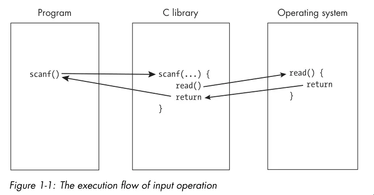
• The OS is often involved in ways users might not suspect. High level library calls actually go through the OS to accomplish tasks such as input/output to the screen:

• Resources are objects that software uses and/or modifies. A program has the privilege to access or modify any of its own resources.
• The OS protects access to a number of resources also known as system resources. These resources include hardware such as the CPU, RAM, screen displays, storage devices, and network connections.
• The OS also protects soft resources such as data structures and files.
• An API typically consists of a collection of function, type, and constant definitions and sometimes variable definitions as well. The OS API provides a means by which user programs can request services. These are system calls.
• System programs make requests for resources and services directly from the operating system or provide functions that higher-level applications can use.
• The term system program also applies to any program that can run independently of the OS and extend its functionality, even if it doesn’t make any direct calls to the API. Examples include the linker, compiler, terminal emulator, etc.
• Ideas key in the design of UNIX:
  • Programmable shells.
  • Users and groups.
  • Privileged and unprivileged instructions.
  • Environments.
  • Files and the directory hierarchy.
  • Device-independent input and output.
  • Processes.
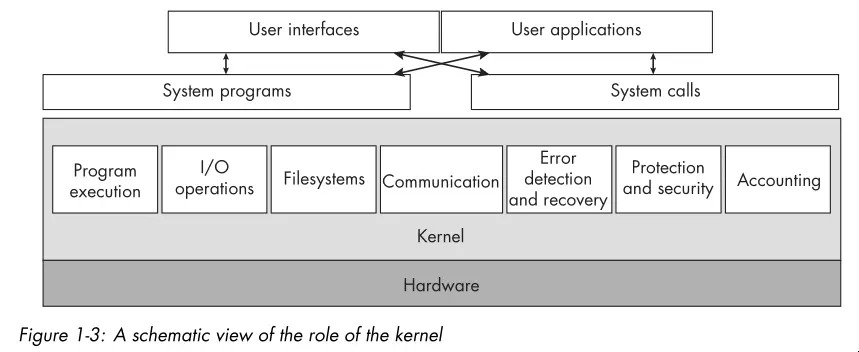
• Below is a high level view of the services a kernel provides:

• The word shell is the UNIX term for a particular type of command line interpreter.
• In modern UNIX systems, a user is any entity that can run programs and own files. The entity need not be an actual person. For example, root, syslog, and lp are nonperson users.
• UNIX requires that the processor support two modes of operation, known as privileged and unprivileged mode. Privileged instructions are instructions that can alter system resources, directly or indirectly. Examples include:
  • Acquiring memory.
  • Changing the system time.
  • Raising the priority of a running process.
  • Reading from or writing to the disk.
  • Entering privileged mode.
• Only the kernel executes privileged instructions.
• When a program runs, one of the steps that the kernel takes before running the program is to make available to it an array of name-value pairs called the environment.
• The directory hierarchy and UNIX’s “everything is a file” philosophy is one of the key features that sets it apart.
• All files have a inode containing metadata (or file status information).
• An ordinary link is a directory entry that points to the inode for a file, but a symbolic link is a file whose contents are just the name of another file. The inode for a symbolic link identifies that file as a symbolic link.
• A process is an instance of a running program.
• A process contains one or more threads. In Linux, a process and a thread are much the same. The key difference is that threads within a process can share resources whereas processes do not share resources with other processes.
• The final section of the chapter gives a good overview of UNIX history as well as its relation to various standards including POSIX.

Chapter 2: Fundamentals of System Programming

• An object library is a file that bundles together, in a structured way, the compiled object code from multiple functions so that programs can call them.
• Many libraries make system calls on behalf of user programs.
• UNIX systems support two kinds of libraries: static and shared.
• A static library is a library whose code gets linked to the program statically, after the program gets compiled, to create the program executable file. In other words, the linker copies the library functions referenced by the program out of the library and inserts them into the program executable file, after which it resolves all unresolved symbols to enable jumps into and out of those functions.
• A shared library is a library whose object code is not copied into the executable, but is instead linked to the program at runtime. Runtime is the interval of time during which the program is actually running. With shared libraries, calls to functions or references to other symbols in the library get linked only when the program actually executes the calls or accesses the symbols for the first time.
• Linux systems have two dynamic linkers: ld.so and ld-linux.so. The former links and loads the old-style executable format know as a.out, and the latter links and loads executables in the modern Executable and Linking Format (ELF).
• There are various binary utilities for examining the contents of libraries and executables:
  • nm: Lists the symbols in an object file.
  • ldd: Lists the shared libraries required by an executable.
  • objdump: Displays information about object files.
  • readelf: Displays information about ELF files.
  • hexdump: Displays the raw byte contents of a file.
  • od: Dumps files in octal and other formats.
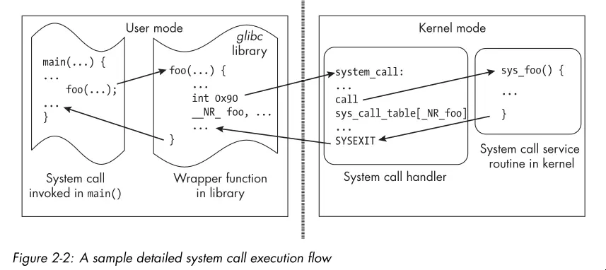
• Often times, libraries call system calls on behalf of user programs. The C library (libc) is the most commonly used library for this purpose. A number of GNU C Library functions are thin wrappers around system calls. The library sets up the registers with the appropriate arguments and then invokes a special CPU instruction that switches the processor from user mode to kernel mode and jumps to a predefined location in the kernel where the system call handler resides. The schematic below illustrates this flow:

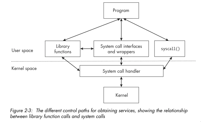
• Some system calls don’t have wrappers in the library, and for those, the programmer has no other choice but to invoke the system call with the syscall() function, passing the system call’s number and arguments.
• The image below demonstrates the different control paths for obtaining kernel services:

• Portability refers to the degree to which your program can run on other computers with little or no modification of the code itself.
• A feature test macro is a macro designed to expose features such as constant and function prototypes in a header file when a program gets compiled.
• Locale is the definition of the subset of a user’s environment that depends on language and cultural conventions.
• When a program works correctly no matter where it’s used and performs input and output consistent with the location in which it’s run, the program has been internationalized. That means accounting for differences such as language, paper sizes, monetary units, time units, and measurement units.
• There’s a good example with explanation of how to use GNU getopt() to parse command line options. It’s worthy of reference over the man page.

Chapter 3: Time, Dates, and Locales

• This chapter mainly demonstrates writing a program that mimics the date utility’s functionality.
• You can modify the TZ environment variable to change the timezone used by time and date functions.
• You can modify the LC_ALL environment variable to change the locale used by time and date functions. LC_ALL overrides all other LC_* variables (see locale(7)).
• A XML like markup language gets used to describe locale information. These XML files pass through a program called localedef to generate binary locale definition files that the C library can use.
• Calling setlocale(LC_ALL, "") causes the program to use the locale specified in the user’s environment. This is the first step in internationalizing a program.
• Many libc functions are locale-aware. For example, strftime() formats date and time strings according to the current locale. Often, setlocale() is all you need to get locale-aware behavior. Otherwise you must use the localeconv() and nl_langinfo() functions to obtain locale-specific information.

Chapter 4: Basic Concepts of File I/O

• The chapter opens with a brief description of umasks. A umask is a set of permissions that the OS uses to restrict the default permissions assigned to newly created files and directories.
• A running process inherits the umask of its parent process or shell. A process can change its umask with the umask() system call.
• Every process gets associated with at least one user ID. On Linux, every process has four user IDs:
  • Real user ID.
  • Effective user ID.
  • Saved set-user-ID.
  • File system user ID.
• The kernel uses the effective user ID when it needs to determine whether to grant a process permission to access a resource.
• The kernel uses the filesystem user ID to determine access to files, but the filesystem user ID is always equal to the effective user ID.
• Normally, when you run a program, the process that’s created gets assigned an effective user ID and real user ID that are both equal to your user ID and thus the same.
• The highest-order bit in a file’s mode is the set-user-ID (SUID) bit. When the SUID bit gets set on an executable file, any process that runs that file gets assigned an effective user ID equal to the owner user ID of the file, rather than the user ID of the user who ran the program.
• A process can access only files for which it has permission to do so. This is determined by the file’s permission and the effective user ID of the running process.
• A process performs file I/O in three steps:
  • Open a connection to the file to read or write.
  • Perform read or writes through that connection.
  • Close the connection to the file.
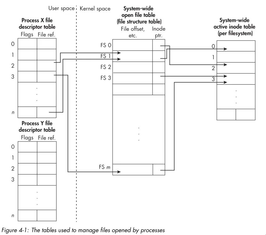
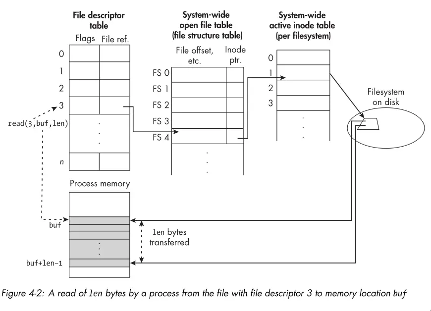
• The following diagram shows how the kernel uses various tables to manage the files opened by processes:

• The open() system call opens a connection to a file and returns a nonnegative integer called a file descriptor that identifies the connection.
• open() takes three arguments:
  • The pathname of the file to open.
  • Flags that determine file creation (read, write, append, create, etc).
  • The file mode (permissions) to use when creating a new file. The umask of the calling process gets applied to the mode permissions.
• close() always gets paired with open() to release the file descriptor and associated resources. Handling close() errors is a tricky subject, see the “Errors When Closing Files” section for some tips.
• The read() system call reads data from a file into a buffer in memory. The drawing below illustrates the process:

• write() works similarly to read(), but in the opposite direction. One of the quirks to keep in mind is that it’s possible that a partial write occurs. In this case, the return value of write() will be less than the number of bytes you requested to write.
• It’s important to know that a call to write() doesn’t guarantee that the data gets written to the physical device. The kernel uses various caching and buffering techniques to optimize I/O performance. To guarantee that data gets physically written, you must use the fsync() or fdatasync() system calls.

Chapter 5: File I/O and Login Accounting

• The lseek() system call repositions the file offset of an open file descriptor. The file offset indicates the position in the file where the next read or write will occur.
• The lseek() system call takes three arguments:
  • The file descriptor of the open file.
  • The offset (in bytes) to which to set the file offset.
  • The reference point from which to set the offset. This can be the beginning of the file, the current file offset, or the end of the file.
• Files can have holes. When reading from a hole, the kernel returns NULL bytes. When writing to a hole, the kernel allocates disk space as needed.
• You can create a hole in a file by using lseek() to set the file offset beyond the end of the file and then writing data at that position.
• A file with holes is a sparse file. The filesystem doesn’t allocate disk space for the holes, which can save disk space. That said, tools like ls will report the apparent size of the file, which includes the holes, rather than the actual disk space used. Other tools like du report the actual disk space used. Worth noting that filesystems allocate disk space in blocks. So a small file with a large hole in the middle may for example end up using two 4KB blocks on disk having then an actual size of 8KB.

Chapter 6: Overview of Filesystems and Files

• Filesystems are the framework for storing files. They organize the entire collection of files, providing both the infrastructure and an interface for accessing them.
• The kernel interacts with disks through device drivers. A device driver is a collection of kernel functions that make a device respond to the various system calls by communicating with the device.
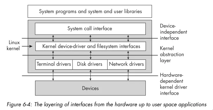
• Below is a graphic showing the layering of interfaces in a typical Linux system:

• Disk partitions or logical disks are subdivisions of physical disks that the OS treats as separate disks.
• Benefits of partitioning a disk includes:
  • More control of file security.
  • More efficient use of the disk.
  • More efficient operation.
  • Selective backup procedures.
  • Improved failure recovery.
  • Reliability.
• The biggest disadvantage of partitioning a disk is that partitions can’t be increased in size.
• Linux supports various filesystems (see filesystems(5)). The ext filesystem and its variants (ext2, ext3, ext4) are the most commonly used.
  • Ext2: The high-performance disk filesystem used by Linux for fixed disks as well as removable media.
  • Ext3: An enhanced version of ext2 that supports journaling.
  • Ext4: A performance upgrade of the Ext3 filesystem.
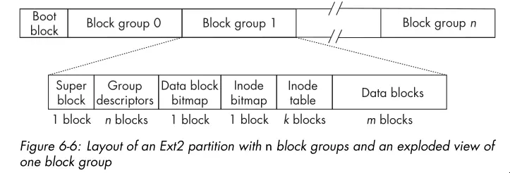
• A modern partition layout may look like this:

• The superblock contains parametric information about the filesystem such as how many inodes it has, the total number of blocks, the block size, the number of reserved and unused blocks, timestamps of various kinds, various flags indicating whether it’s read-only or locked, information about the system’s mount status, and much more.
• The group descriptors store information about the group such as the address of the starting block of each other component of the block group, how many blocks in the group are in use, how many are free, and so on.
• The data block bitmap is a bitmap with 1 bit for every data block in that group. If the block is in use, the bit is 1, and if free, the bit is 0.
• The inode bitmaps serves a similar purpose for inodes as the data block bitmap does for data blocks. It contains a bit for each inode in the inode table, which indicates whether it’s in use or free.
• The inode table stores all inodes for files whose data is in the block group.
• A filesystem has to provide methods that the kernel can call so that it can provide its services to user programs. Such methods include functions to create files, to read and write data, to retrieve file properties, to move the file offset, and so on.
• Lets think about the steps the kernel takes to create a file (ignoring error handling):
  • It checks whether the filename is valid and whether the filename doesn’t exist already in the given directory.
  • It checks whether the process has permission to create a file in this directory.
  • It acquires a new inode for the file.
  • It fills in the inode with the file status.
  • It creates a directory entry in the directory with the inode number and filename.
• Writing data requires:
  • Allocating data blocks for the file and storing the file data into these blocks.
  • Recording the addresses of the data blocks in the inode.
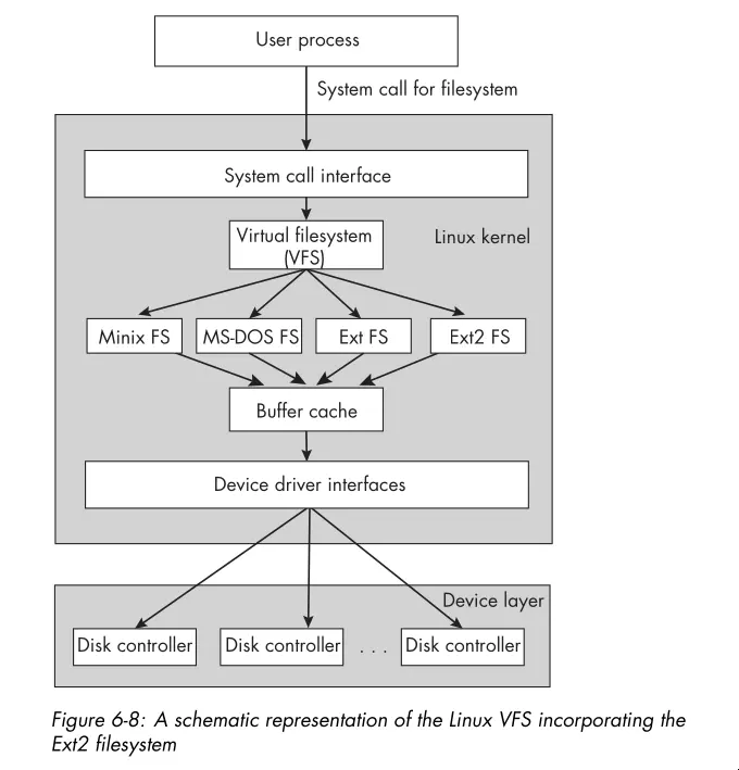
• Linux has a Virtual Filesystem (VFS) layer which defines a set of functions that every filesystem must implement. This interface includes operations associated with three kinds of objects: filesystems, inodes, and open files. Here’s a schematic view of the VFS layer:

• The Linux kernel provides a few system calls for obtaining the metadata associated to files, including stat(), lstat(), and statx(). It also provides a separate set of calls for accessing filesystem metadata, including statfs(), and the C library provides the POSIX-conforming statvfs().

Chapter 7: The Directory Hierarchy

• A directory consists of a set of (inode number, filename) pairs called links.
• Directories are never empty because every directory has two unique entries: . and ...
• You create and modify directories only by specific system calls, unlike regular files, which you create by calling open() and creat().
• You can traverse directories by first getting a pointer to a directory stream via opendir(), then reading entries from the stream with readdir(). The entries themselves only guarantee the presence of the entry filename and inode number. See readdir(3) for more details on the other entries.
• The scandir() function reads the contents of a directory into an array of pointers to dirent structures. You provide a optional filter function to select which entries to include and a optional comparison function to sort the entries. It’s handy for filtering and sorting a single directory level.
• When you mount a filesystem to a particular directory, the original contents of that directory become inaccessible until the filesystem gets unmounted.
• A process can recognize when a directory dir is a mount point because the device ID of the directory’s parent, say, parent is different from that of dir. This is because dir is the root of the mounted filesystem and parent is a node on the filesystem to which it’s attached.
• Due to mounting, to uniquely identify a file, you must know both the inode number and the device ID. This is because different filesystems can have files with the same inode number.
• The nftw() function performs a depth-first traversal of a directory tree, starting at the specified pathname. It calls a user-defined callback function for each file and directory it encounters. This is useful for performing operations on all files in a directory tree, such as calculating the total size of files or searching for files with specific attributes. It has options for controlling the traversal behavior as well.
• There’s also an fts family of functions for traversing directory trees. They provide more control and flexibility than nftw(). The API is arguably worse. That said, GNU utilities like grep, chmod, and rm use fts functions for directory traversal.

Chapter 8: Introduction to Signals

• Signals serve as a form of notification about some event or condition of importance that’s sent to a recipient.
• In UNIX, signals are essentially software interrupts; they’re empty messages delivered to a process that interrupt its normal instruction cycle.
• Many signals are like hardware interrupts in that they can occur at any time, independent of what a process is doing when they arrive. The kernel is almost always the source of the signal.
• Sometimes, one process can send a signal to another, and a process can send a signal to itself.
• Signals carry with them no information other than the signal type. The signal type is an integer that identifies the signal. For example, SIGINT has a signal number of 2, and SIGTERM has a signal number of 15.
• There are a number of sources of signals, including:
  • User
  • Kernel
  • Hardware Exceptions
  • Other Processes
• A process that’s sent a signal may not be executing at the time the signal got sent. Until it resumes execution and the signal is actually delivered to it, the signal is pending for that process.
• The kernel will never deliver a duplicate signal to a process’s signal queue. You can think of the signal queue as a set of bits.
• Processes also have the ability to temporarily block certain types of signals by defining a signal mask.
• A signal is delivered to a process when it responds to the signal in one of the following ways:
  • The process explicitly ignores the signal. You can’t ignore some signals.
  • The process executes a signal handler.
  • The process accepts the default action associated with the signal. These include:
    • Terminate
    • Ignore
    • Stop
    • Core Dump
    • Continue
• signal(7) and signal.h(7posix) provide all the information you would need about signals on any Linux system.
• A processes signal disposition is the set of actions that the process takes in response to signals. The signal disposition for a particular signal can be changed by the process with the sigaction() system call.
• There’s also an older system call: signal(2). You shouldn’t use it. That said, if you encounter it in the wild, beware that its semantics can vary between BSD and System V UNIX systems. In System V, the signal handler gets reset to the default after the first signal gets delivered, but in BSD, the signal handler remains in place until explicitly changed. You can toggle between the two via feature test macros.
• You can interrupt a system call via a signal. Some system calls get restarted after the signal handler returns, but others will not (for example, sleep). You can read more in signal(7).
• You can use CLI utilities like kill and pkill to send processes signals. Despite the name, by default, kill sends the SIGTERM signal. You can send any signal you find in the man pages with the -s option.
• You can send signals to other processes or process groups programmatically using kill(3). Only those processes with a matching real or effective user ID can send signals to a process. The kill() function takes two arguments: the PID of the target process and the signal number to send. The first argument to kill() dictates its behavior. See the man page for examples.
• You can also raise signals from within a process with the raise() function. This is equivalent to sending a signal to yourself with kill().
• Blocking a signal means informing the kernel to hold onto that signal for a short time until you’re ready for it. You can view signal blocking as putting as short-term hold on signal delivery while your program performs some actions that you don’t want interrupted. If you want the signal blocked for a long time, it would be better to use signal() to set its disposition to SIG_IGN.
• You can use the sigprocmask() system call to block and unblock signals. These work in conjunction with the sigset_t data type. See the sigsetops man page for more info.
• Blocked signals are not queued. If you block a signal and it’s generated multiple times, only one instance of it gets delivered when that signal is unblocked.
• POSIX requires that when a signal gets unblocked with a call to sigprocmask(), if it’s ending, the signal gets delivered to the process immediately, before the sigprocmask() call returns.
• If you want to atomically update the signal mask of the process and suspend it until a signal that terminates or triggers a registered handler gets delivered, use the sigsuspend() system call. The expected way to use sigsuspend() is in conjunction with sigprocmask(). The program blocks signals, executes a critical section of code, and calls sigsuspend() to unblock the signals and wait for delivery of a signal. This still requires writing a signal handler for the signals.
• The sigwait() and sigwaitinfo() system calls are useful when you want to write programs that respond to specific signals in a synchronous way, meaning without writing signal handlers that run whenever the signals get sent, but instead responding to them within the program’s ordinary functions.
• The sigaction() system call replaces the use of signal() for installing signal handlers and controlling their behavior. The programmer specifies how the handler will respond when multiple signals get sent to a program while it’s executing a signal handler.
• If you handle a synchronous signal, your handler must terminate the program or raise SIGTERM to terminate the program. Otherwise, the instruction that caused the signal gets re-executed after the handler returns creating a loop.
• The signum and ucontext_t arguments of the sigaction() signal handler are often not used. The siginfo_t structure contains information about the signal and its source. What fields it contains depends on the signal type and source. For more information, consult the sigaction man page or POSIX.1-2024 specification.
• The section describing the behaviors of the sa_flags field is worth re-reading if you’re programming with sigaction().
• See the signal-safety man page for more information about which function are safe inside signal handlers.

Chapter 9: Timers and Sleep Functions

• Most computers have a designated hardware clock called the real-time clock (RTC) that keeps wall clock time. Among the RTCs, there’s one that’s backed up by a battery while the computer is off or in a low power state so that it keeps its time.
• Many computers also have a hardware device called a programmable interval timer (PIT). The PIT issues an interrupt, called a timer interrupt, whenever it times out. The PIT is a hardware timer that continues to generate interrupts at the same rate as long as the machine is on. Linux kernels typically program the PIT to issue interrupts about once every millisecond, a frequency of 1,000 Hz.
• The interval between adjacent PIT interrupts is a tick.
• A third type of timekeeping device is the time stamp counter. Linux systems sometimes use this hardware counter for higher-precision timing. The oscillator in this device has a much higher frequency than the PIT.
• A fourth type of timer is the High Precision Event Timer (HPET). These timers container internal counters that they update at least once every 10 microseconds, meaning a frequency of at least 100 KHz.
• The system clock is a software clock, which means that time gets recorded and updated entirely by software. On reboots, the kernel initializes the system clock by either reading time from the RTC or, if it has a network connection, by getting it from a network time service such as an NTP server. Once initialized, the system clock stores the time since the Epoch. The system clock gets updated every time it receives an interrupt from the PIT.
• A jiffy is the unit of time between adjacent PIT interrupts. The resolution of software timers depends on the value of a jiffy. A timer can’t be more accurate than the length of a jiffy. On some newer systems, timer system calls aren’t based on jiffies but instead on high-resolution timers such as the HPETs.
• In the world of high-resolution sleep functions you have nanosleep() and clock_nanosleep(). The latter is the preferred function since you can specify the clock and set timers based on absolute time. The ability to set absolute timers is important to avoid the problem of timer drift. See nanosleep(2) for more information on timer drift.
• The alarm() system call is a simple timer that sends the SIGALRM signal to the process after a specified number of seconds have elapsed. It’s not a high resolution timer, and it’s not suitable for most timing purposes.
• An interval timer is a timer that expires at regular intervals until it’s explicitly canceled. The setitimer() system call provides interval timers. The modern timer API uses timer_gettime(), timer_settime(), and friends.
• You’ll have to read the section in this book or the man pages to understand the interval timer API. They overload many of the parameters.
• Timer overruns are timer expiration event notifications that get generated but never delivered or accepted by the process. Kernel scheduling or other system activities can cause this to happen. You can get a count of overruns with timer_getoverrun().
• POSIX defines at least eight real time signals that you can use for timer expiration notifications. In general, they range from SIGRTMIN to SIGRTMAX. These signals are different than the standard signals in that they get queued by the kernel and lower valued signals have higher priority.

Chapter 10: Process Fundamentals

• Modern UNIX systems introduced the concept of a process group as an abstraction of a job. The motivation for this feature is to simplify the way in which a pipeline gets terminated with a signal.
• There are system calls for getting/setting a process’s process group ID. See man setpgid(2) and getpgid(2).
• A process group has a leader process whose PID is the same as the process group ID. The leader process is the first process in the group. When a process creates a child process, the child process inherits the process group ID of its parent, so it becomes a member of the same process group.
• A session or login session is the collection of all processes created directly or indirectly when you log in. Formally, a session is a collection of process groups, and every process group belongs to exactly one session. Each process has a unique session ID (SID) that identifies the session to which it belongs.
• The primary purpose of a session is to organize processes around their controlling terminals. The controlling terminal for a process is the terminal that delivers signals to the process when the user enters certain key combinations or sequences. When a user logs in, the kernel creates a session, places all processes and process groups of that user into the session, and links the session to the terminal as its controlling terminal.
• A daemon is a process that has no controlling terminal and usually runs until the computer gets powered off.
• You can changed a processes’ session ID with setsid().
• Processes fall into one of two categories: foreground or background. The idea is that foreground processes get connected to the terminal, whereas background processes aren’t. Every session can have multiple process groups, but at most one of them can be a foreground group; the others must be in the background.
• Foreground processes can read input from the terminal and receive signals sent via the keyboard directly. Background processes can’t read input from the terminal and don’t receive signals unless sent via kill.
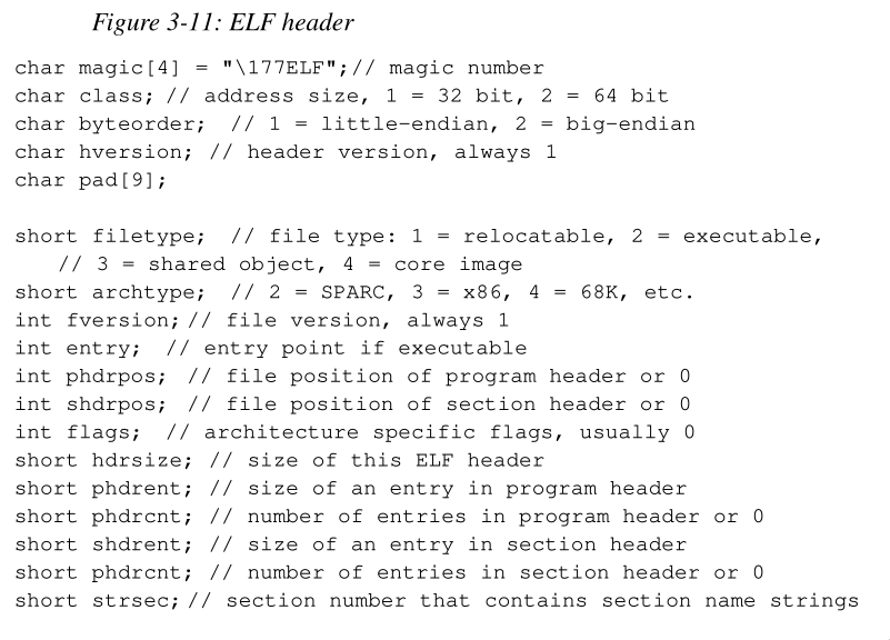
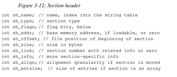
• There’s a brief section on the ELF format. You should checkout the Linkers and Loaders notes for more information on the ELF format and how executables get loaded.
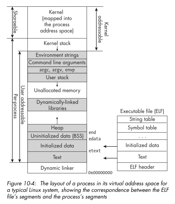
• Here’s the layout of a process in its virtual address space:

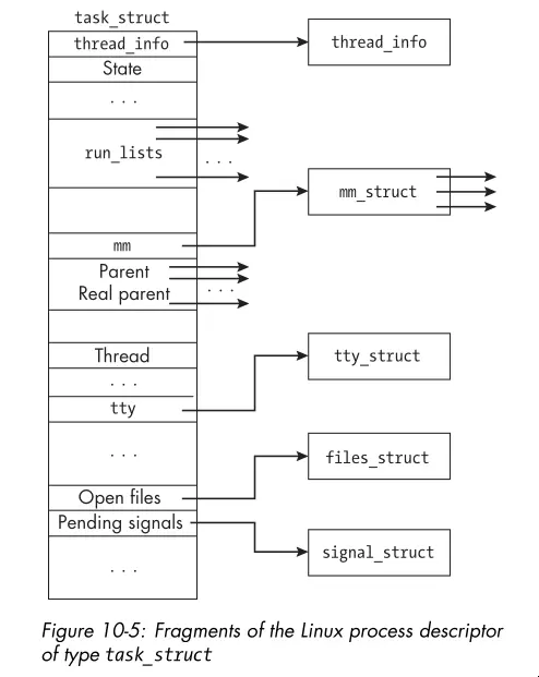
• The Linux process descriptor is a kernel data structure that contains all the information about a process that the kernel needs to manage it. The task_struct structure represents the process descriptor in Linux. Here’s a graphic showing just a handful of the fields:

• You can’t access most of the information in the process descriptor from user space through the system call interface.
• /proc is pseudo-filesystem that provides an interface to kernel data structures. It contains a directory for each running process, named by its PID, and within each process directory, there are files that provide information about the process. Some useful files include:
  • cmdline: The complete command line for the process.
  • comm: The executable file that the process is executing.
  • cwd: A symbolic link to the process’s current working directory.
  • environ: The initial environment set when the program got started. It might have changed after program start. The strings are NULL separated.
  • exe: A symbolic link containing the pathname to the executed command.
  • fd: A subdirectory containing links to each open file descriptor.
  • io: Input/output statistics for the process.
  • maps: The currently mapped memory regions and their access permissions. This shows information such as where the heap and stack and linked libraries get loaded.
  • stat: Status information about the process. This file isn’t as easily read as status but gets used by ps.
  • statm: Memory usage, measured in pages.
  • status: Similar status information to that in stat, but easier to read.

Chapter 11: Process Creation and Termination

• The fork() system call creates a new process by duplicating the calling process. The child process gets an exact copy of the parent’s memory, file descriptors, and other resources, but it has a unique PID and its own execution context.
• Some things that don’t carry over to the child process include:
  • The set of pending signals.
  • Any per-process timers.
  • The child’s PID is unique and different from any active PGID.
  • Message queues, semaphores, and shared memory segments are not inherited by the child process.
• Open file descriptors get shared between the parent and child. The child’s descriptor is even at the same offset. If the child moves the offset or the parent moves it, the other process sees the change! You need to synchronize access to avoid unexpected behavior. This leads to a form of IPC.
• You want to use fork() in your programs. vfork() is a variant of fork() that’s deprecated and more of historical note. clone() and its variants are Linux specific. clone() is a more flexible system call that you use to control which resources get shared between the parent and child processes.
• exit() terminates the calling process and returns an exit status to the parent process. When exit() gets called, these events take place in order:
  • All functions registered to run with atexit() run in the reverse order in which they got registered.
  • All file streams opened through the Standard I/O Library get flushed and closed.
  • The kernel’s _exit() function gets called, passing the status argument of exit() to it.
• Child processes inherit the exit functions registered by the parent when fork() created them.
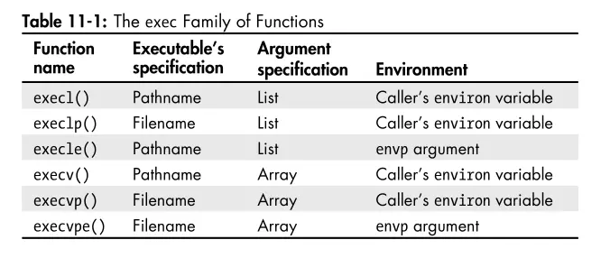
• The execve() system call replaces the current process image with a new process image specified by the pathname argument. The ve stands for vector because the argv and envp arguments are vectors of strings. The other exec functions do the same thing but provide slightly different interfaces for convenience. The table below summarizes the differences:

• The wait() system call suspends the calling process until one of its child processes terminates. It returns the PID of the terminated child and stores the child’s exit status in the location pointed to by the status argument.
• The waitpid() system call is a more flexible version of wait(). You specify which child process to wait for and provide options for controlling the behavior of the waiting process. Worth reading the man page for more details.
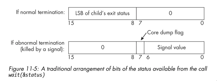
• The W*() macros tell you the exit status returned by wait() and waitpid(). You can determine whether the child process terminated normally or abnormally, and if it terminated normally, what its exit status was. If it terminated abnormally, you can determine whether it was due to a signal and which signal caused the termination.
• Below is an image illustrating the format of the exit status:

• The system() function is a convenient way to execute a shell command from a C program. It takes a string argument that contains the command to execute. The system() function creates a child process, invokes the shell to execute the command, and waits for the command to complete before returning. Check out the man page. In general, you should avoid using system() in production code because it can be a security risk.

Chapter 12: Introduction to Interprocess Communication

• Data gets exchanged between processes either through a shared storage medium or by transferring it through some channel that the operating system manages.
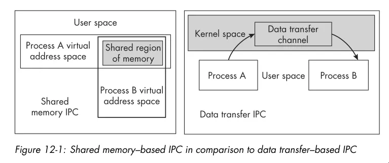
• Shared memory is one form of IPC. The memory region used for sharing is in the processes’ address spaces. The kernel is not involved in the transfer of data to and from this memory.
• There’s also data transfer IPC. The kernel gets involved in the transfer of data. Think pipes, sockets, and message queues.
• See the graphic below for a illustration of the differences between the two forms of IPC:

• Unlike shared memory IPC, data transfer IPC methods provide the mutual exclusion needed to prevent race conditions, freeing the programmer from having to prevent them explicitly. That said, data transfer IPC methods are slower than shared memory IPC.
• Message queues support the reading and writing of messages. Only one message gets read at a time. When a message gets read, it’s removed from the queue. Message queues are not the same as the FIFO IPC mechanism!
• Semaphores are another IPC method. They’re usually used for synchronization between processes. You can increment a semaphore sem_post() and decrement it sem_wait(). The operations are atomic. If one process attempts to decrement a semaphore whose value is zero, it gets blocked until another process increments it.
• You can get an overview of the POSIX shared memory interface by reading shm_overview(7). A shared memory object encapsulates the metadata associated with the memory region created by the kernel. On Linux, it’s created in an in-memory tmpfs filesystem and has a name visible in the /dev/shm directory.
• If writing a program in C/C++ that will use the POSIX shared memory API, give the “Shared Memory API” section a read.
• When working with shared memory, be careful not to store pointers to memory in one or more processes’ address space. Those addresses are invalid when dereferenced by the other processes. Instead, you should use offsets to store the locations of data in the shared memory region.
• You must protect access to shared memory with some form of synchronization, such as semaphores to prevent race conditions if that region of memory is both read and written.
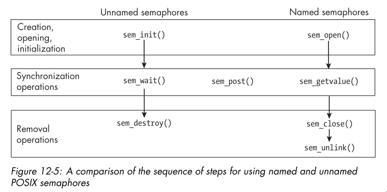
• The sem_overview(7) man page gives a overview of POSIX semaphores. There are two types of POSIX semaphores: named and unnamed:
  • Names Semaphore: Has a name of the form /name similar to a shared memory region name. Two processes operate on the same named semaphore by passing that name to the sem_open() function.
  • Unnamed Semaphore: Has no name. You must create it in an address space common to all processes or threads that operate on it. This means that, for processes, it must be in a shared memory object shared by the processes.
• The functions supported by named and unnamed semaphores look like this. Not shown are the wait() and post() functions which are common to both.

• You’ll probably see unnamed semaphores more often since if two processes are synchronizing access to a shared memory region, it makes sense to put the unnamed semaphore in that region.
• The mq_overview(7) man page contains a good summary of POSIX message queues and refers you to the man pages that describe how to use them.
• POSIX message queues are not necessarily first-in-first-out queues because each message is a assigned a priority. It’s a priority queue.
• Message queues are handy for communicating data synchronously or in contexts where polling is okay. Asynchronous communication is possible with message queues, but it’s more complicated to set up. The asynchronous side of the API alerts a process that a first message has arrived in the message queue. It’s not meant for alerting a process of every message that arrives.

Chapter 13: Pipes and FIFOs

• FIFOs is the POSIX term for a named pipe. A typical pipe requires that the processes on both ends of the pipe share a common ancestor. A FIFO has no such requirement.
• A pipe is a unidirectional data channel for interprocess communication. Here are the key features of a pipes/FIFOs:
  • Creating a pipe returns two file descriptors.
  • Pipes transmit byte streams.
  • Pipes preserve the order of the data written to them.
  • Reads from the pipe drain the pipe.
  • Reads are blocking by default.
  • Pipes have limited capacity.
  • Writes of at most PIPE_BUF bytes are atomic.
• The read and write semantics on pipes get complicated. See the tables on page 652 for a clear summary of the possible scenarios.
• The dup() system call duplicates an existing file descriptor using the lowest numbered unused file descriptor. Here’s a snippet illustrating the idea:

int pipefd[2];
if ( pipe(pipefd) == -1 )
// Handle error and exit.
--snip--
close(1);
/* Close descriptor 1, making it lowest unused descriptor.*/
dup(pipefd[1]); /* Now descriptor 1 points to the write end of the pipe. */
close(pipefd[1]); /* Close the pipe's write end descriptor.
*/

• The code has a problem in that a race condition exists. The problem is that if a program has any signal handlers and a signal arrives after the closing of descriptor 1 but before the call to dup(), the signal handler might open a new file descriptor, using slot 1, and dup() will not duplicate the descriptor into standard output. This race condition is the reason why dup2() exists. dup2(fd, fdtoreplace) atomically performs the two steps of closing fdtoreplace and replacing it with fd.
• Named pipes are unlike unnamed pipes in that:
  • They exist as directory entries in the file system and therefore have associated permissions and ownership.
  • They get used by processes that are not related to each other.
  • They get created and deleted at the shell level or through the system API.

Chapter 14: Client-Server Applications and Daemons

• The word daemon is from Greek mythology and refers to a lesser god that did helpful tasks for the people it protected.
• A daemon is a process that runs in the background without a controlling terminal.
• A daemon can use the syslog logging service to log its messages.
• The important part of daemons is that they execute without an associated terminal or login shell, usually waiting for an event to occur.
• Daemon names often but not always end in “d.”
• These are the steps a process must take to turn itself into a daemon:
  • Putting itself in the background.
  • Making itself a session leader.
  • Registering its intent to ignore SIGHUP.
  • Executing its code as a new child of the existing process.
  • Changing the current working directory to /.
  • Clearing the umask.
  • Closing any open file descriptors.
• An iterative server is a server that services the requests from its clients in an iterative fashion, meaning one after another.
• A concurrent server is one that forks a separate process (or perhaps a thread) to handle each request.

Chapter 15: Introduction to Threads

• In modern Linux, each user level thread, meaning threads the program creates, get assigned to a kernel scheduling entity called a lightweight process.
• The functions in the pthreads API fall into one of four groups:
  • Thread Management
  • Mutexes
  • Condition Variables
  • Synchronization
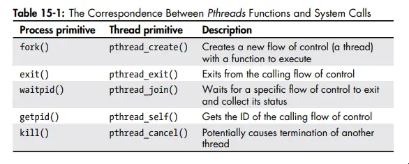
• Here’s the correspondence between pthreads functions and system calls:

• Worth taking a second look at page 712 to see what resources are and are not shared between threads.
• You don’t always have to join threads, you can also detach them. You can’t join detached threads, and their resources get automatically released when they terminate. You can detach a thread with pthread_detach() or by setting the thread’s detach state to PTHREAD_CREATE_DETACHED when you create it with pthread_attr_setdetachstate().
• Exceeding the default stack limit of a thread is possible even on modern machines. Threads stacks are usually no more than 8KB by default. If the stack limit gets exceeded, the program will terminate, possibly with corrupted data. You can explicitly allocate more stack space for a thread with pthread_attr_setstacksize(). Or you can allocate on the heap.
• The interaction between signals and threads is a mess. See page 727 for an explanation with examples.

Chapter 17: Alternative Methods of I/O

• You can poll most resources by setting the O_NONBLOCK flag on the file descriptor.
• Non-blocking I/O is a form of polling. Whether the read/write operation succeeds, you’re making many system calls and often wasting CPU cycles.
• Worth noting for the O_NONBLOCK flag, this flag has no effect for regular files and block devices; that is, I/O operations will block when device activity occurs, regardless of whether you set O_NONBLOCK.
• In signal driven I/O, a process informs that kernel in advance that it wants to get a signal whenever it’s possible to read or write a given open file descriptor, and it establishes a signal handler to catch this signal.
• Signal driven I/O is a edge triggered notification method enabled by setting the O_ASYNC flag on the file descriptor. It’s only available in Linux and BSD and so isn’t portable. This is arguably not async I/O either because you at best get a notification that data is ready but the data has yet to be transferred to the process address space.
• POSIX AIO provides a API for async communications that mirrors the usual read, write, etc API (see aio(7)). The POSIX AIO implementation lives in glibc. The implementation doesn’t scale well since each operation spawns a new user level thread.
• You can receive AIO completion notifications via signals or threads. Additionally, the AIO API includes functions for suspending and cancelling AIO operations.
• I/O multiplexing is a service provided by the kernel allowing processes to monitor multiple file descriptors for possible I/O activity. This service associates with the select(), poll(), and epoll() system calls. epoll() is Linux only and is the most efficient of the three albeit hardest to use. The book describes select() in detail.
• Read the man pages and also select_tut(2) for more information and examples.

Chapter 18: Terminals and Terminal I/O

• People don’t use actual terminal devices anymore; instead, they use software-emulated terminals on bitmapped graphical displays.
• Terminal canonical mode is the default mode of terminal input processing. In this mode, the terminal driver provides line editing and other features. The terminal driver buffers gather input until a newline character gets sent, at which point it makes the input available to the reading process.
• Programs like Emacs, vi, and less put the terminal into a noncanonical mode called raw mode, in which the terminal passes all input to the process with no processing.
• The behavior of the terminal gets controlled entirely by a software component called a terminal driver. A terminal driver consists of two subcomponents:
  • A terminal device driver
  • A line discipline
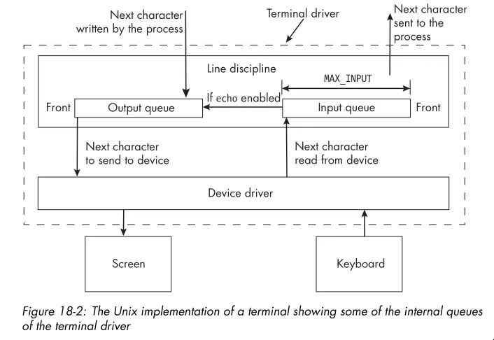
• The terminal device driver’s main function is to transfer characters to and from the terminal device; it’s the software that talks directly with the physical terminal or the terminal emulator and the line discipline at the other.
• For a terminal, the line discipline is the software that does the processing of input and output. It manages several queues, including an input queue and an output queue for the terminal driver.
• The image below shows the relationship between the terminal device driver and the line discipline:

• The stty command can both display and alter terminal characteristics. With the -a option, you can see most of the settings for the terminal connected to the shell in which you invoked the command.
• There are several categories of terminal attributes:
  • Special Characters: Characters that get used by the driver to cause specific actions to take place, such as sending signals to the process or erasing characters or words or lines. Examples include CTRL-C for sending SIGINT and CTRL-D for sending an end-of-file indication.
  • Special Settings: Variables that control the terminal in general, such as its input and output speeds and dimensions. These include the rows, cols, min, and time values.
  • Input Settings: Operations that process characters coming from the terminal. This includes changing their case, converting carriage returns to newlines, and ignoring various characters like breaks and carriage returns.
  • Output Settings: Operations that process characters sent to the terminal. Output operations include replacing tab characters with the appropriate number of spaces, converting newlines to carriage returns, carriage returns to newlines, and changing case.
  • Local Settings: Operations that control how the driver stores and processes characters internally. For example, echo is a local operation, as is processing erase and line-kill characters.
  • Combination Settings: Combinations of various settings that define modes such as cooked mode, raw mode, and sane mode.
• Input switch names always begin with an i and output switch names begin with o.
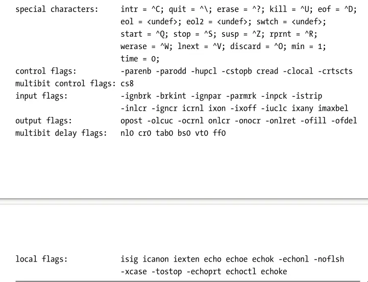
• Below is a capture showing examples of the different terminal attributes reported by stty -a:

• See termios(3) for more information about the terminal attributes and how to manipulate them programmatically.

In this article, you’ll learn how to improve performance, enable bluetooth, and more in NixOS. The goal is to get you closer to a full desktop experience in NixOS. Configurations provided in this article come from NixOS Discourse and the NixOS Wiki. It’s worth checking out both resources for more information and help.

If you don’t have a NixOS installation on your PC, you can experiment with these configurations in a virtual machine. Check out NixOS QEMU VM Setup for guidance. Keep in mind that some configurations may have no effect on a VM or may require added configuration at VM launch time. The rest of this article assumes you have a vanilla NixOS installation and are familiar with editing /etc/nixos/configuration.nix and rebuilding your system via sudo nixos-rebuild switch.

Temperature Control (Intel CPUs)

To proactively prevent overheating of Intel CPUs, you can use the thermald service. From the thermald man page:

thermald is a Linux daemon used to prevent the overheating of platforms. This daemon monitors temperature and applies compensation using available cooling methods.

By default, it monitors CPU temperature using available CPU digital temperature sensors and maintains CPU temperature under control, before HW takes aggressive correction action.

Add the following line to your NixOS configuration file to enable thermald:

services.thermald.enable = true;

Performance Governor

To balance performance and power consumption, you can set the CPU frequency scaling using the auto-cpufreq service. Using the configuration below, you can save power when on battery and maximize performance when plugged in:

services.auto-cpufreq.enable = true;
services.auto-cpufreq.settings = {
  battery = {
     governor = "powersave";
     turbo = "never";
  };
  charger = {
     governor = "performance";
     turbo = "auto";
  };
};

You can verify the current governor policy across all cores with the following command:

cat /sys/devices/system/cpu/cpu*/cpufreq/scaling_governor

Audio

By default, NixOS uses PipeWire for audio management. Here’s a basic audio configuration using PipeWire with ALSA and PulseAudio support:

security.rtkit.enable = true;

services.pipewire = {
  enable = true;
  alsa.enable = true;
  alsa.support32Bit = true;
  pulse.enable = true;
};

You may also want to install pavucontrol for graphical volume control:

environment.systemPackages = with pkgs; [
  pavucontrol
];

Bluetooth

To enable Bluetooth support in NixOS, you can use the following configuration:

hardware.bluetooth = {
  enable = true;
  powerOnBoot = true;
};

You can verify that the Bluetooth service is running with:

systemctl status bluetooth

Additionally, you may want to install packages to assist with Bluetooth management:

environment.systemPackages = with pkgs; [
  bluez
  bluez-tools
  blueman
];

blueman provides a graphical interface for managing Bluetooth devices that integrates with most desktop environments. bluez-tools includes useful command-line utilities such as bluetoothctl.

Docker

To enable Docker support in NixOS, you can use the following configuration:

virtualisation.docker.enable = true;

Additionally, you must add your user to the docker group:

users.users.<USERNAME> = {
  extraGroups = [ "wheel" "docker"];
};

Be sure to replace <USERNAME> with your actual username.

sudo Without a Password

If you like to live dangerously, you can configure sudo to not require a password for your user by adding the following to your NixOS configuration:

security.sudo.extraRules= [
    {
      users = [ "<USERNAME>" ];
      commands = [
        { command = "ALL" ;
          options= [ "NOPASSWD" ];
        }
      ];
    }
];

Be sure to replace <USERNAME> with your actual username.

GPG Agent

GPG agent conveniently manages your GPG keys and can also handle SSH keys. To enable the GPG agent with SSH support and a curses-based pinentry program, add the following to your NixOS configuration:

programs.gnupg.agent = {
  enable = true;
  enableSSHSupport = true;
  pinentryPackage = pkgs.pinentry-curses;
};

You can search NixOS packages for alternative pinentry options.

OpenSSH

You can enable and configure the OpenSSH server in NixOS with the following:

services.openssh.enable = true;
services.openssh.ports = [ 54446 ];
services.openssh.settings.PasswordAuthentication = false;

This configuration enables the OpenSSH server, sets it to listen on port 54446, and disables password authentication for improved security.

You’ll need to add your public SSH key to your user’s authorized_keys file. You can do that as follows:

  users.users.<USERNAME> = {
    openssh.authorizedKeys.keys = [
        "<YOUR_SSH_PUBLIC_KEY>"
    ];
  };

Be sure to replace <USERNAME> with your username and <YOUR_SSH_PUBLIC_KEY> with your SSH public key.

XServer + Desktop Manager + Window Manager

To set up a graphical environment in NixOS, you can enable the X server, a desktop manager, and a window manager. Here’s an example configuration using lightdm as the desktop manager and i3 as the window manager:

services.xserver = {
  enable = true;
  exportConfiguration = true;
  windowManager.i3.enable = true;

  displayManager =  {
    lightdm.enable = true;
    lightdm.greeters.gtk.enable = false;
    lightdm.greeters.slick.enable = true;
  };
};
services.displayManager = {
  defaultSession = "none+i3";
};
security.pam.services = {
  i3lock.enable = true;
  i3lock-color.enable = true;
};

You’ll want to further configure the window manager, status bars, etc. for your user. A follow-up article will cover how that’s done using the home-manager module.

Conclusion

Here’s the full configuration in one single snippet for easy copy-pasting:

{ config, pkgs, ... }:

{
  services.thermald.enable = true;

  services.auto-cpufreq.enable = true;
  services.auto-cpufreq.settings = {
    battery = {
       governor = "powersave";
       turbo = "never";
    };
    charger = {
       governor = "performance";
       turbo = "auto";
    };
  };

  security.rtkit.enable = true;

  services.pipewire = {
    enable = true;
    alsa.enable = true;
    alsa.support32Bit = true;
    pulse.enable = true;
  };

  environment.systemPackages = with pkgs; [
    pavucontrol
    bluez
    bluez-tools
    blueman
  ];

  hardware.bluetooth = {
    enable = true;
    powerOnBoot = true;
  };

  virtualisation.docker.enable = true;

  users.users.<USERNAME> = {
    extraGroups = [ "wheel" "docker"];
    openssh.authorizedKeys.keys = [
        "<YOUR_SSH_PUBLIC_KEY>"
    ];
  };

  security.sudo.extraRules= [
      {
        users = [ "<USERNAME>" ];
        commands = [
          { command = "ALL" ;
            options= [ "NOPASSWD" ];
          }
        ];
      }
  ];

  programs.gnupg.agent = {
    enable = true;
    enableSSHSupport = true;
    pinentryPackage = pkgs.pinentry-curses;
  };

  services.openssh.enable = true;
  services.openssh.ports = [ 54446 ];
  services.openssh.settings.PasswordAuthentication = false;

  services.xserver = {
    enable = true;
    exportConfiguration = true;
    windowManager.i3.enable = true;

    displayManager =  {
      lightdm.enable = true;
      lightdm.greeters.gtk.enable = false;
      lightdm.greeters.slick.enable = true;
    };
  };
  services.displayManager = {
    defaultSession = "none+i3";
  };
  security.pam.services = {
    i3lock.enable = true;
    i3lock-color.enable = true;
  };
}

Integrate these configurations into your existing configuration.nix file as needed. As always, refer to NixOS Packages and NixOS Options for more information on available packages and configuration options.

This article will walk you through the process of running NixOS in a QEMU virtual machine (VM) on a Linux host system. Basic nix configuration to help with connectivity to the VM from the host is also included.

This article assumes you’re on a Arch Linux host system. Instructions may vary with regards to package installation on other distros, but the rest of the steps should be largely identical. Additionally, your machine must support virtualization and have it enabled in the BIOS/UEFI settings.

Installing QEMU and QEMU Utilities

You’ll need the QEMU emulator package for your host architecture along with the qemu-img utility to create disk images. On Arch Linux, you can install these packages in a single command:

sudo pacman -S qemu-full

Verify the installation by running:

qemu-system-x86_64 --version
qemu-img --version

Tip: qemu-full is a large package that includes support for multiple architectures. If you want to save space, you can install only the emulator for your host architecture (for example, qemu-system-x86_64 for x86_64 hosts). If you go this route, remember to additionally install the qemu-img package.

Downloading the NixOS ISO

You can download the latest NixOS ISO from the NixOS download page. For a first time user, it’s best to download a “Graphical ISO image”. Graphical installation ISOs contain a desktop environment with an installation wizard.

Installing NixOS to a Virtual Disk

Create a disk image for your NixOS VM. The following command creates a 30GB QCOW2 image.

qemu-img create -f qcow2 nixos-vm.qcow2 30G

The base installation comfortably fits within 10GB. That said, give yourself at least another 20GB for app installs.

Create a bash script in the same directory as your QCOW2 image called start-nixos-vm.sh. Add the following content to boot the NixOS installation ISO:

#!/bin/bash

qemu-system-x86_64 \
    -m 6144 \
    -smp 3 \
    -drive file=nixos-vm.qcow2,format=qcow2 \
    -cdrom /path/to/nixos-graphical-25.11.941.c97c47f2bac4-x86_64-linux.iso \
    -boot d \
    -net nic \
    -net user,hostfwd=tcp::2222-:22 \
    -enable-kvm

You may want to adjust the following parameters based on your system and preferences:

Option	Description
-m 6144	Allocates 6GB of RAM to the VM.
-smp 3	Allocates 3 CPU cores to the VM.
-cdrom <ISO_PATH>	Path to the NixOS ISO downloaded earlier.
-enable-kvm	Optional feature for better performance. See the Arch Wiki’s KVM article for more information.

Run the start-nixos-vm.sh script to boot into the installation ISO. The install wizard should launch automatically. Follow the on-screen instructions to complete the installation. Once done, shut down the VM.

Booting into NixOS

Modify the start-nixos-vm.sh script to boot from the virtual disk instead of the installation ISO. Update the script as follows:

#!/usr/bin/env bash

qemu-system-x86_64 \
    -m 6144 \
    -smp 3 \
    -drive file=nixos.qcow2,format=qcow2 \
    -net nic \
    -net user,hostfwd=tcp::2222-:22 \
    -enable-kvm

Remember to adjust the -m and -smp values as needed.

Running the script once more should boot you into your newly installed NixOS VM. From here, you can begin your NixOS journey from the comfort of a virtual machine.

Bonus: SSH Access

With the -net user,hostfwd=tcp::2222-:22 option in the QEMU command, you can SSH into your NixOS VM from the host machine. But first, you’ll need to enable SSH in your configuration.nix. Follow these steps to connect via SSH:

1. Run your NixOS VM.
2. Edit your nix config:

sudo nano /etc/nixos/configuration.nix`.

3. Uncomment or add the line services.openssh.enable = true;.
4. Rebuild your NixOS configuration:

sudo nixos-rebuild switch`.

5. On the host machine, run the following command replacing <USERNAME> with your NixOS username:

ssh -p 2222 <USERNAME>@localhost

The keyball44 is a 40% split keyboard with a built-in trackball. It supports custom keymaps through QMK firmware. As a first step to programming the board, you modify a keymap.c file. It’s easy to make mistakes when editing the keymap.c file, especially when dealing with multiple layers and complex keycodes. That’s where keyball44-viz comes in. keyball44-viz is a command-line tool written in Rust that parses a keymap.c file and generates an SVG visualization of the keyboard layout.

Taking a Look at keymap.c

The snippet below defines six layers for the keyboard, including a base layer, symbol layer, number layer, navigation layer, function layer, and trackball layer. Each layer gets defined using the LAYOUT_universal macro, which maps key positions to keycodes.

const uint16_t PROGMEM keymaps[][MATRIX_ROWS][MATRIX_COLS] = {
    // Base Layer
  [0] = LAYOUT_universal(
    KC_TAB   , KC_Q     , KC_W     , KC_E     , KC_R     , KC_T     ,                                        KC_Y     , KC_U     , KC_I     , KC_O     , KC_P     , KC_BSPC   ,
    KC_LCTL  , KC_A     , KC_S     , KC_D     , KC_F     , KC_G     ,                                        KC_H     , KC_J     , KC_K   , LT(5, KC_L), KC_SCLN  , KC_ENT  ,
    KC_LSFT  , KC_Z     , KC_X     , KC_C     , KC_V     , KC_B     ,                                        KC_N     , KC_M     , KC_COMM  , KC_DOT   , KC_SLSH  , KC_RSFT  ,
                  MO(4),KC_LALT,KC_LGUI     ,MO(3),KC_SPC,                                        MO(1),MO(2), KC_RALT,     _______  , MO(5)
  ),

    // Symbol Layer
  [1] = LAYOUT_universal(
    _______ ,  KC_GRV   ,S(KC_BSLS), _______  , KC_QUOT  ,S(KC_QUOT),                                        _______  ,S(KC_LBRC),S(KC_RBRC), KC_LBRC  , KC_RBRC  , _______  ,
    _______ , S(KC_1)   ,  S(KC_2) , S(KC_3)  , S(KC_4)  , S(KC_5)  ,                                         S(KC_6) , S(KC_7)  , S(KC_8)  , S(KC_9)  , S(KC_0)  , _______  ,
    _______ ,  _______  , _______  , _______  , _______  , _______  ,                                         _______ , _______  , _______  , _______  , KC_BSLS  , _______  ,
                _______,_______,_______     ,_______,_______,                                     _______,_______,_______,   _______  , _______
  ),

    // Number Layer
  [2] = LAYOUT_universal(
    _______ , S(KC_GRV) , _______  , _______  , _______  , _______  ,                                         _______ , KC_MINUS ,S(KC_MINUS), KC_EQL  , S(KC_EQL), _______  ,
    _______ , KC_1      , KC_2     , KC_3     , KC_4     , KC_5     ,                                         KC_6    , KC_7     , KC_8      , KC_9    , KC_0     , _______  ,
    _______ , _______   , _______  , _______  , _______  , _______  ,                                        _______  ,_______   , _______   ,_______  ,_______   ,_______   ,
                _______,_______,_______     ,_______,_______,                                     _______,_______,_______,   _______  , _______
  ),

    // Navigation Layer
  [3] = LAYOUT_universal(
    KC_ESC  , _______   , _______  , _______  , _______  , _______  ,                                        _______  , KC_PGUP  , KC_PGDN   , KC_HOME , KC_END   , KC_DEL   ,
    _______ , _______   , _______  , _______  , _______  , _______  ,                                        _______  , KC_LEFT  , KC_DOWN   , KC_UP   , KC_RIGHT , S(KC_INSERT),
    _______ , _______   , _______  , _______  , _______  , _______  ,                                        _______  ,_______   , _______   ,_______  ,_______   ,_______   ,
                _______,_______,_______     ,_______,_______,                                     _______,_______,_______,   _______  , _______
  ),

    // Function Layer
  [4] = LAYOUT_universal(
    _______ , KC_F11    , KC_F12   , _______  , _______  , _______  ,                                        _______  , _______  , KC_PSCR   , KC_SCRL , KC_PAUSE , _______  ,
    _______ , KC_F1     , KC_F2    , KC_F3    , KC_F4    , KC_F5    ,                                        KC_F6    , KC_F7    , KC_F8     , KC_F9   , KC_F10   , _______  ,
    _______ , KC_CAPS   , KC_NUM   , _______  , _______  , _______  ,                                        _______  , _______  , _______   , _______ , _______  , _______  ,
                _______,_______,_______     ,_______,_______,                                     _______,_______,_______,   _______  , _______
  ),

    // Trackball Layer
  [5] = LAYOUT_universal(

    _______  , AML_TO   , AML_I50  , AML_D50  , _______  , _______  ,                                        _______  , _______  , _______  , _______ , _______ , _______  ,
    _______  , _______  , _______  , _______  , _______  , SCRL_DVI ,                                        _______  , KC_BTN1  , KC_BTN2  , _______ , _______  , _______  ,
    _______ , _______  , _______  , _______  , _______  , SCRL_DVD ,                                        CPI_D1K  , CPI_D100 , CPI_I100 , CPI_I1K  , _______  , KBC_SAVE ,
                  QK_BOOT  , KBC_RST  , _______  ,        _______  , _______  ,                   _______  , _______  , _______       , KBC_RST  , QK_BOOT
  ),
};

In the example, the keymaps at each layer contain whitespace meant to help developers visualize the layout. Not all keymaps you come across online will look this neat. Additionally, small screens/line wrapping can still make a well organized keymap file difficult to read. A basic visual representation can help you validate the layout before putting in the effort to build and flash the firmware.

Visualizing the Keymap

This image is a visualization of the keymap previously defined. A separate keyboard diagram matching the keyball44 layout gets drawn for each layer. Keys get labeled according to their assigned keycodes. Each layer has a distinct color scheme to differentiate them.

You can move keys around in your keymap.c file and regenerate the SVG to see how the changes affect the layout. Just pass keyball44-viz your keymap.c file for processing. The whole process takes just a few seconds, making it easy to iterate on your design.

Usage

You can build keyball44-viz from source using Cargo. Alternatively, you can download precompiled binaries for both Windows and Linux x86_64 from the releases page on GitHub.

Usage is straightforward. Run the tool from the command line providing the path to your keymap.c file:

keyball44-viz path/to/keymap.c

The tool will output a keymap.svg file in the current directory. You can view the SVG in a browser. For a full list of options, run keyball44-viz --help.

Workplace monitoring is a practice that has seen a significant rise since 2020 (a totally anecdotal claim). Maybe you’ve worked with one of these managers that constantly checks if you’re active on Discord, Teams, insert other company chat app. A lot of people work from home these days. It’s not uncommon for folks to want to get out of their chair and stretch their legs, grab a coffee, or just take a quick break from the screen. That break often means an idle system. If you got a whacko boss that monitors status, you might find yourself in hot water for being “inactive” for a few minutes.

It usually doesn’t take much more than moving the mouse a little to keep the status showing active. That’s where a tool like bz (pronounced “busy”) comes in handy. bz is a simple CLI tool written in Rust that simulates mouse movement at regular intervals to keep your system from going idle.

How It Works

bz works by moving your mouse cursor from the location it’s currently at, to the center of the screen, and back again. How often the mouse moves is configurable via a command line argument (default is every 5 seconds). There’s also an option to click at the end of each interval, which can be useful for some applications that require more than just movement to stay active. The demo below shows bz in action:

{{< video src=“/posts/2025/busy/busy.mp4” type=“video/mp4” preload=“auto” >}}

It doesn’t do anything fancy. Just a simple back and forth motion with optional clicks. You can stop the program at any time by pressing the ESC key (the terminal doesn’t doesn’t have to be in focus for the program to stop).

Here’s the core part of the code that handles the mouse movement:

// Spawn main busy loop thread that moves the mouse
let busy_handle = std::thread::spawn(move || -> Result<()> {
    let mut enigo = Enigo::new(&Settings::default())?;
    let (width, height) = enigo
        .main_display()
        .context("Failed to get main display size")?;
    let interval = Duration::from_secs(args.update_interval);
    let mut start = enigo.location().context("Failed to get mouse location")?;
    let mut end = (width / 2, height / 2);

    // Continue moving mouse until ESC is pressed
    while rx.try_recv().is_err() {
        enigo
            .move_mouse(end.0, end.1, Coordinate::Abs)
            .context("Failed to move mouse")?;
        if args.click {
            enigo
                .button(Button::Left, Direction::Click)
                .context("Failed to click mouse")?;
        }
        // Swap start and end positions for next iteration
        std::mem::swap(&mut start, &mut end);

        // Check if ESC was pressed or if the sender was dropped (listen thread errored)
        match rx.recv_timeout(interval) {
            Ok(_) | Err(mpsc::RecvTimeoutError::Disconnected) => break,
            Err(mpsc::RecvTimeoutError::Timeout) => continue,
        }
    }
    Ok(())
});

The enigo crate does the heavy lifting. Enigo provides a cross-platform API for moving and clicking the mouse.

You’ll notice that the code runs in a thread that’s on the receiving end of a channel. A second thread listens for a global escape key press and signals the busy loop thread to stop when the user wants to exit the program. The rdev crate makes it easy to listen for global key events. Here’s the code:

fn handle_esc_key(event: Event, tx: mpsc::Sender<()>) {
    if let EventType::KeyPress(Key::Escape) = event.event_type {
        tx.send(()).expect("Failed to send ESC key event");
    }
}

// Spawn keyboard listener thread to detect ESC key press
std::thread::spawn(move || -> Result<()> {
    listen(move |event| handle_esc_key(event, tx.clone()))
        .map_err(|e| anyhow::anyhow!("Error: {:?}", e))?;
    Ok(())
});

That’s pretty much the whole program. One thread listens for the escape key, while the other runs a loop that moves the mouse at regular intervals until it receives a signal to stop.

Usage

You should ideally build bz from source using the usual cargo build --release command. If you like to live dangerously, download a pre-built binary from the releases page on GitHub. The release contains pre-built binaries for Linux and Windows x86_64 platforms.

bz is a command line application, so you should open up a terminal to run it. That’s true on both Windows and Linux. That said, on Windows you can double click the executable in Explorer to run it with the default settings. It’ll popup a console window that you can minimize or just leave on screen.

Remember, you can stop the program at any time by pressing the ESC key from anywhere on the desktop.

Disclaimer

Use this tool at your own risk. If you do use it, try not be a complete goon and abuse it. Silly people abusing software is how you got here in the first place!

This post includes the notes made while reading the book titled “Linkers and Loaders” by John Levine. The book includes exercises that have you incrementally build a linker. A partial implementation is available on GitHub: mild.

Chapter 1: Linking and Loading

• The basic job of any linker or loader is simple: it binds more abstract names to more concrete names, which permits programmers to write code using the more abstract names.
• Linkers assign relative addresses within a program. Loaders do final relocation to assign actual addresses in memory.
• Program loading is the process of copying a program from secondary storage into main memory. This may involve allocating storage, setting protection bits, or arranging for virtual memory to map virtual addresses to disk pages.
• Relocation is the process of assigning load addresses to the various parts of the program, adjusting the code and data in the program to reflect the assigned addresses.
• Symbol resolution is just as the name suggests: take a symbol name and resolve it to an address in the code or a library.
• There’s a lot of overlap between linker and loader responsibilities. In general, the loader loads the program into memory. The linker performs symbol resolution. Either can do relocation. It’s also possible to have an all in one tool that does all three functions.
• Both linkers and loaders patch object code.
• Linking is a two pass process. The linker takes as its input a set of input object files, libraries, and perhaps command files, and produces as its result an output object file, and perhaps ancillary information such as a load map or a file containing debugger symbols.
• Each input contains segments, contiguous chunks of code or data that are merged in the output file. Each input file also contains at least one symbol table.
• You can import symbols. These are names that must be present in one of the other input files. You can export symbols. This makes the symbol name visible to code in the other input files.
• All linkers support object code libraries. A library is just a collection of object files. The linker resolves undefined names in the input files by looking at the library’s object code for exported names that match.
• With dynamic linking, the linker leaves hints for the loader of the symbols required and what libraries they’re found so the loader can patch the code at runtime.
• Typically, you invoke the linker through the compiler driver.
• The various linkers can take commands. This includes command line switches and special scripts which can give the programmer control of where sections get loaded.

Chapter 2: Architectural Issues

• Two aspects of hardware architecture affect linkers: program addressing and instruction formats. One thing the linker does is modify addresses and offsets both in data memory and in instructions.
• The aspect of the Abstract Binary Interface that most often affects the linker is the definition of a standard procedure call.
• Usually addresses are byte aligned. This means that if you have an $N$ byte datum, its address should have at least $log_2(N)$ least significant zero bits.
• Unaligned accesses can degrade performance on some systems. On others, unaligned access leads to faults.
• The instruction format is of concern to the linker. Specifically those instructions surrounding addressing data. Instructions can be of fixed or variable length. They usually consist of an opcode followed by operands.
• Every ABI defines a standard procedure call sequence using a combination of hardware-defined call instructions and conventions about register and memory use.
• Within a procedure, data addressing falls into four categories:
  • A caller can pass arguments to the procedure.
  • Local variables get allocated within the procedure and freed before the procedure returns.
  • Local static data gets stored in a fixed location in memory and is private to the procedure.
  • Global static data gets stored in a fixed location in memory and can be referenced from many different procedures.
• There’s usually a frame pointer pointing to the return address of the procedure. There’s also a stack pointer pointing to the top of the stack. Arguments to the procedure are at negative offsets to the frame pointer (higher memory addresses). Local variables are at positive offsets to the frame pointer (lower memory addresses). The OS usually sets the initial stack pointer before a program starts.
• The compiler generates a table of pointers to local and global static data. The address of that table gets loaded into a register. You require another register to calculate offsets from that base address.
• Within some architectures, the linker must create a table of pointers that captures static data across all modules/object files. In other systems, procedures within a module have their own table. A register gets loaded with the procedure’s table address before that procedure gets called.
• There’s a bootstrapping problem here where the first procedure called needs to have its static data table pointer set up. This is usually done by the linker via some special code.
• Modern computers support virtual memory. On these machines, paging hardware divides the program’s address space into fixed size pages, typically 4KB in size. The same hardware divides the physical memory into page frames of the same size. The hardware contains page tables with an entry for each page in the address space.
• A page table entry can contain the real memory page frame for the page, or flag bits to mark the page “not present.” When a program attempts to use a page that isn’t present, hardware generates a page fault. Page faults get handled by the OS which can copy content from disk into a free page frame. Moving data back and forth between disk and memory makes it seem like the system has more memory than it actually does (virtual memory).
• Page tables are usually hierarchical. The hardware divides the virtual address into three parts: a top-level page table index, a second-level page table index, and an offset within the page. The hardware uses the top-level index to find the second-level page table, then uses the second-level index to find the page table entry. This can vary by architecture.
• Every application runs in an address space defined by a combination of the computer’s hardware and OS. The linker or loader needs to create a runnable program that matches that address space.
• Address space layouts vary from system to system. Some systems have a single address space where the OS and all programs share the same address space. Others partition the address space and allocate a free chunk large enough to hold the program.
• Many systems provide a memory mapping mechanism for mapping a file into the address space of a program. The OS sets up the page tables so that when the program accesses a page in the mapped region, the OS loads the page from the file on disk. Policies for mapping files include read-only, read-write, and copy on write (COW). COW is interesting because it means changes made in the address space are only visible to that process.
• Shared libraries often use position independent code (PIC). This means you can load the code at any address in memory without modification. Only data pages still usually contain pointers which need relocation, but since data pages map COW anyway, there’s little sharing lost.
• Embedded systems pose special challenges for linkers and loaders. They often have address spaces that divide into regions for ROM, RAM, and peripherals. The linker needs to know about these regions and place code and data appropriately.
• On some embedded systems, there’s references to on-chip and off-chip memory. The linker needs to know which addresses are on-chip and which are off-chip so it can place code and data appropriately. You can also use tricks to copy code or data from slow memory to fast memory as needed. To do this, you have to tell the linker “put this code at location X but link it as though it’s at location Y.” The code gets copied from X to Y at runtime.

Chapter 3: Object Files

• An object file contains five kinds of information:
  • Header Information: Overall information about the file, such as the size of the code, name of the source file it derives from, and creation date.
  • Object Code: Binary instructions and data generated by a compiler or assembler.
  • Relocation: A list of the places in the object code that have to be fixed up when the linker changes the addresses of the object code.
  • Symbols: Global symbols defined in this module, imported symbols from other modules or defined by the linker.
  • Debugging Information: Other information about the object code not needed for linking but of use to a debugger. This includes source file and line number information, local symbols, and descriptions of data structures.
• A object file may be:
  • Linkable: Used as input by a link editor or linking loader.
  • Executable: Loads into memory and runs as a program.
  • Loadable: Loads into memory as a library along with a program.
  • A combination of the three is also possible.
• An object file could be all binary code. This is how MS DOS .COM files work.
• In UNIX, the a.out format introduces separate sections for instructions and data. Instructions live in a .text section. Data lives in a .data section. Uninitialized data lives in a .bss section. Read-only text sections are shareable amongst multiple processes.
• The a.out format also includes a header. The header contains sizes of the different sections. Also at the start of the header is a magic number that tells the loader how to load the file into memory.
• On a BSD system using the QMAGIC load format, the layout in memory looks like:
  • The object exists as a file on disk. The text section of that file will be loaded as read-only pages into the address space of the process. The data sections load as read-write pages that are COW.
  • The first page of the address space is blank to catch NULL pointer dereferences.
  • The header and text section follow next in the address space.
  • The data section follows next with the BSS section concatenated on the end.
  • The heap follows the BSS section with stack pages allocated some ways down.
  • Note, all sections are page aligned meaning text/data sections get rounded up to the next page boundary.
• The key thing with the BSD formats is that they assign a fresh address space to each process so that every program loads at the same logical address. These object formats are simple because they can be directly loaded to memory. No need for a linker.
• Executable Link Format (ELF) is a modern object file format used on many UNIX-like systems. ELF comes in three slightly different flavors: relocatable, executable, and shared object.
• Compilers and assemblers create relocatable files. The linker needs to process these before they can run.
• Executable files have all relocation done and all symbols resolved except perhaps shared library symbols that get resolved at runtime.
• Shared objects contain both symbol information for the linker and directly runnable code for runtime.
• Compilers, assemblers, and linkers treat an ELF file as a set of logical sections described by a section header table, while the system loader treats the file as set of segments described by a program header table.
• Here’s a capture of the ELF header with descriptions:

• A relocatable or shared object is a collection of sections defined in section headers. The notes that follow apply to relocatable ELF files.
• Each section contains a single type of information, such as program code, read-only data, read-write data, relocation entries, or symbols.
• Every symbol in a module is relative to a section.
• Here’s a capture of the section header table with descriptions:

• Here’s a list of sections and their attributes:
  • .text which is type PROGBITSwith attributes ALLOC+EXECINSTR. It’s the equivalent of a.out’s text section.
  • .data which is type PROGBITS with attributes ALLOC+WRITE. It’s the equivalent of a.out’s data section.
  • .rodata which is type PROGBITS with attribute ALLOC. It’s read-only data hence no WRITE attribute.
  • .bss which type NOBITS with attributes ALLOC+WRITE. The BSS section takes no space in the file, hence NOBITS, but gets allocated at runtime, hence ALLOC.
  • .rel.text, .rel.data, and .rel.rodata each of which type REL or RELA. The relocation information for the corresponding text or data section.
  • .init and .fini which are type PROGBITS with attributes ALLOC+EXECINSTR. These are similar to .text, but they execute when the program starts up or terminates. These factor in with C++ which has global data with executable initializers and finalizers.
  • .symtab and .dynsymb types SYMTAB and DYNSYM regular and dynamic linker symbol tables. The dynamic linker symbol table is ALLOC since it loads at runtime.
  • .strtab and .dynstr are both type STRTAB, a table of name strings, for a symbol table or section names for the section table.
• Here’s a capture of an ELF symbol table entry with descriptions:

• A ELF executable has the same general format as a relocatable ELF file, but the data gets arranged so that the file can map into memory and run. The notes that follow describe executable ELF files.
• An ELF executable contains a program header that follows the ELF header. The program header defines the sections of the file that get mapped to process memory.
• Here’s a capture of the ELF program header with descriptions:

• An executable has a handful of segments, a read-only one for the code and read-only data, and read-write one for the read-write data. All the loadable sections pack into the appropriate segments so the system can map the file with one or two operations.
• An ELF shared object contains all the baggage of a relocatable and an executable. It has the program header table at the beginning, followed by the sections in the loadable segments, including dynamic linking information. Following sections comprising the loadable segments are the relocatable symbol table and other information that the linker needs while creating executable programs that refer to the shared object, with the section table at the end.

Chapter 4: Storage Allocation

• A linker or loader’s first major task is storage allocation. Once storage gets allocated, the linker can proceed to subsequent phases of symbol binding and code fixups.
• Storage layout is a two-pass process since the location of each segment can’t get assigned until the sizes of all segments that logically precede it are known.
• Linkers will usually take the text segments of all modules and merge them together one after the other. Space gets allocated to house the merged text segments making sure to respect the alignment requirements of the target. The same gets done for data and BSS segments where data always follows text and BSS follows data.

• When you add paging, the same process happens with the distinction that the first data page follows the last text page. BSS gets interpreted as data so some BSS data actually lives on data pages.
• With C++ there’s a duplicate removal problem created by virtual function tables, templates, and extern inline functions. There are several solutions:
  • Live with the duplication. Downside here is significant code bloat for large projects.
  • Compilers generate the duplicate code and linkers are “smarter” in the sense they can identify and remove duplication. Usually “link once” sections get emitted by the compiler. The linkers see these sections and discard all but the first one. Some linkers will inspect the content of the sections before discarding. This isn’t perfect since type information gets lost at this point. For example, a template taking pointer to int and one taking pointer to float may look identical at the binary level.
• C++ also exacerbates the initializer/finalizer problem. In C++, you have static variables. The variables may have constructors and destructors. The linker needs to arrange for the constructors to run before main() and destructors to run after main() exits. The common solution is to create special sections .init_array and .fini_array which contain pointers to the constructors and destructors. The startup code runs the constructors in order before calling main(). The exit code runs the destructors in reverse order after main() returns. Within the init and fini sections, there’s further ordering. Often library routines need to run before constructors and vice versa for the cleanup code. In this case, there might be several init/fini sections ordered by the linker appropriately.
• The last source of linker-allocated storage is the linker itself. When a program uses shared libraries, the linker creates segments with pointers, symbols, etc. for runtime support of the libraries. Once these segments get created, the linker allocates storage for them the same way it does for the other segments.
• Many linkers support control scripts that let the programmer control storage allocation. The scripts can specify the order of segments, their alignment, and even their absolute addresses. This is especially useful for embedded systems where code and data need to go in specific memory regions.

Chapter 5: Symbol Management

• Symbol management is the linker’s key function. All linkers handle symbolic references from one module to another.
• Each input module includes a symbol table. The symbols includes:
  • Global symbols defined and perhaps referenced in the module.
  • Global symbols referenced but not defined in this module (called externals).
  • Segment names which are usually also considered to be global symbols defined to be at the beginning of the segment.
  • Non-global symbols usually for debuggers and crash dump analysis. These aren’t symbols needed for the linking process, but sometimes they’re mixed in with global symbols so the linker has to at least skip over them.
  • Line number information to tell source language debuggers the correspondence between source lines and object code.
• Within a linker, there’s one symbol table listing the input files and library modules, keeping the per-file information. A second symbol table handles global symbols, the ones that the linker has to resolve among input files. A third table may handle intra-module debugging symbols, although more often than not the linker need not create a full-fledged symbol table for debug symbols.
• On the first pass, the linker reads each input file’s symbol table and stores each table in some program data structure. The linker also creates a single global symbol table for every symbol referenced or defined in any input file.
• During the second pass, the linker resolves symbol references as it creates the output file.
• The output file usually contains a symbol table of its own. This is because the output file can be a relocatable object file.
• Some linkers output special symbols such as etext, edata, and end to mark the end of the text, data, and BSS segments respectively. The system sbrk() routine uses end to find the start of the heap. A similar strategy gets used with constructors and destructors so that the program start up stub can call a list of routines on startup and shutdown.
• Names get mangled for three reasons:
  • Avoiding name collisions
  • Name overloading
  • Type checking
• Many object formats can qualify a reference as weak or strong. A strong reference must get resolved while a weak reference may get resolved if there’s a definition, but it’s not an error if it’s not. Linker processing of weak symbols is much like that for strong symbols except that at the end of the first pass an undefined reference to one isn’t an error.
• Debugging symbols are sometimes included in the output module sometimes placed in a separate file. The debug info often includes line number information as well as names, types, and locations of program variables.
• With ELF in particular, the DWARF debugging format is common. You can strip the object of its debug info using the strip command.

Chapter 6: Libraries

• The term libraries in this chapter refers to collections of object files that get included as needed in a linked program (statically linked libraries).
• UNIX linker libraries use an “archive” format which you can use for collections of any type of files, although in practice it’s used just for object files.
• The archive consists of a text header with an extension for long names and a directory called /.
• a.out archives store the directory in a member called __.SYMDEF. Which is the first member of the archive following the header. In contrast, COFF/ELF files name the directory /.
• A COFF/ELF directory looks like this: The first four byte value is the number of symbols. What follows is an array of file offsets of archive members, and a set of NULL terminated strings. The first offset points to the member that defines the symbol named by the first string, and so forth.
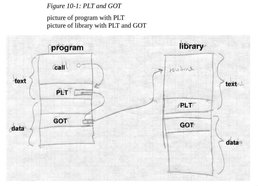
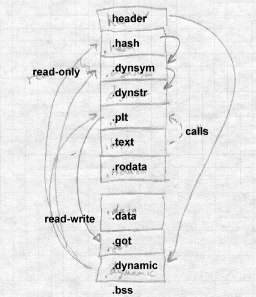
• For COFF and ELF files, ar is the utility which creates a symbol directory if any of the members appears to be an object module.
• Library search happens during the first linker pass after the individual input files get read. If the library or libraries have symbol directories, the linker reads in the directory and checks for each symbol in the linker’s symbol table. For each undefined symbol, the linker includes that symbol’s file from the library. It’s not enough to mark the file for later loading; the linker has to process the symbols in the segments in the library file just like those in an explicitly linked file. The segments then go in the segment table, and the symbols, both defined and undefined, go in the global symbol table.
• Linkers almost always process the objects and libraries in the order they appear on the command line. This means that if two libraries A and B form a circular dependency, you have to list one of them twice on the command line: A -> B -> A. The problem becomes worse when there’s three or more libraries exhibiting this behavior.
• Weak symbols are symbols that get resolved only if they’re referenced. Unreferenced weak symbols are not defined and this is not considered an error. This is useful for libraries where you have optional routines that get used only if needed.

Chapter 7: Relocation

• Relocation refers to both the process of adjusting program addresses to account for non-zero segment origins, and the process of resolving references to external symbols, since the two are frequently done together.

• Hardware relocation enables the operating system to give each process a separate address space that starts at a fixed known address, which makes program loading easier and prevents buggy programs in one address space from damaging programs in other address spaces.

• Software linker or loader relocation combines input files into one large file that’s ready to get loaded into the address space provided by hardware relocation, frequently with no load-time fixing up at all.

• UNIX systems never relocate ELF programs although they do relocate ELF shared libraries. That is, programs get linked so that they load at a fixed address which is usually available, and no load-time relocation gets done except in the unusual case that the standard address is already in use by something else.

• Load-time relocation is simple compared to link-time relocation. At link time, different addresses get relocated different amounts depending on the size and locations of the segments. At load time, on the other hand, the entire program is invariably treated as a single big segment for relocation purposes, and the loader needs only to adjust program addresses by the difference between the nominal and actual load addresses.

• The requirements of relocation and symbol resolution are slightly different. For relocation, the number of base values is small, the number of segments in an input file, but the object format has to permit relocation of references to any address in any segment. For symbol resolution, the number of symbols is far greater, but the only action the linker needs to take with the symbol is to plug the symbol’s value into a word in the program.

• Relocation falls into two categories: absolute and PC-relative. Absolute relocation means adding the base address of the related segment to the address. PC-relative relocation means adjusting an offset relative to the program counter to reflect the distance between the instruction and its target.

• The linker must implement a different number of relocation strategies depending on the target architecture. This is due to how the different instructions encode addresses and offsets.

• Relocation tables are usually stripped from the output object. If the relocation table isn’t stripped, then the output object is a relocatable. Load-time relocation is possible with a relocatable object.

• Many object formats define special segment formats that require special relocation processing.

Chapter 8: Loading and Overlays

• Loading is the process of bringing a program into memory so it can run.
• On most modern systems, each program gets loaded into a fresh address space, which means that all programs get loaded at a known fixed address and can be linked for that address.
• Here’s the basic process:
  • Read enough header information from the object file to find out how much address space you need.
  • Allocate that address space in separate segments if the object format has separate segments.
  • Read the program into the segments in the address space.
  • Zero out any BSS space at the end of the program if the virtual memory system doesn’t do so automatically.
  • Create a stack segment if the architecture needs one.
  • Set up any runtime information such as program arguments or environment variables.
  • Start the program.
• Load time relocation is sometimes done and is usually a simple process. Suppose the program gets linked to load at address 0. Then if the program actually gets loaded at 15000, then all fixup address just need to have 15000 added to them.
• Load time relocation can present a performance problem because code loaded at different virtual addresses can’t usually get shared between address spaces since the fixups for each address space are different. One popular solution is position independent code (PIC).
• The idea is to separate the code from the data and generate code that won’t change regardless of the address at which it’s loaded. That way the code can shared among all processes with only data pages being private to each process.
• The advantages of PIC are straightforward: it makes it possible to load code without having to do load-time relocation and to share memory pages of code among processes even though they don’t all have the same address space allocated.
• The possible disadvantages are slowdown at load time, in procedure calls, in function prolog and epilog, and overall slower code.
• At load time, although the code segment of a PIC file needn’t get relocated, the data segment does. In large libraries, the table of contents or Global Offset Table may be large and it can take a long time to resolve all the entries.
• PIC code is bigger and slower than non-PIC. The slowdown varies by architecture.
• Overlays are mostly obsolete in world a with virtual memory. What’s important to know is that overlays originated the important technique of “wrapping” call instructions in the linker to turn a simple procedure call into one that did more work. Linkers use wrapping in a variety of ways. The most important is dynamic linking to link a called routine in a library that may not have been loaded yet.

Chapter 9: Shared Libraries

• A program that uses a shared library depends on having that shared library available when the program runs. In this case, printing an error message is all you can do.
• With static shared libraries, symbols get bound to addresses at link time. This means that the library must not change or it will break linked programs.
• The most difficult aspect of shared libraries is address space management. Each shared library occupies a fixed piece of address space in each program in which it’s gets used.
• Creating a shared library involves three steps:
  • Determine at what address the library’s code and data will load.
  • Scan through the input library to find all the exported code symbols.
  • Make up the jump table with an entry for each exported code symbol. The jump table is just a sequence of jump instructions to the actual code.
  • If there’s initialization or a loader routine at the beginning of the library, compile or assemble that.
  • Create the shared library. Run the linker and link everything together into one big executable format file.
  • Create the stub library. Copy the necessary symbols from the newly created shared library, reconcile those symbols with the symbols from the input library, create a stub routine for each library routine, then compile or assemble the stubs and combine them into the stub library.

Chapter 10: Dynamic Linking and Loading

• Benefits of dynamic linking include:
  • Easier to create than static linked shared libraries.
  • Easier to update than static linked shared libraries.
  • The semantics of dynamically linked shared libraries can be much closer to those of unshared libraries.
  • Dynamic linking permits a program to load and unload routines at runtime, a facility that can otherwise be difficult to provide.
• Disadvantages of dynamic linking include:
  • The runtime performance cost of dynamic linking is greater than static linking. This is because a large part of the linking process gets done each time the program runs.
  • Every dynamically linked symbol used in a program gets looked up in a symbol table and resolved.
  • Dynamic libraries are also larger than static libraries since the dynamic ones have to include symbol tables.
  • There’s also an administrative cost. It’s easy to install a shared library that breaks existing programs.
• ELF shared libraries can get loaded at any address so they invariably use position independent code so that the text pages of the file need not be relocated and get shared among multiple processes.
• ELF linkers support PIC code with a Global Offset Table (GOT) in each shared library that contains pointers to all the static data referenced in the program. The dynamic linker resolves and relocates all the pointers in the GOT. This can be a performance problem mostly for large libraries.
• Similar to the GOT which points to static data in the SO, the Procedure Linkage Table (PLT) contains pointers to all the external functions called by the program. The PLT permits lazy evaluation, that is, procedure addresses don’t get resolved until the first time they’re called.

• An ELF dynamically linked file contains all the linker information that the runtime linker will need to relocate the file and resolve any undefined symbols:
  • The .dynsym section, the dynamic symbol table, contains all the file’s imported and exported symbols.
  • The .dynstr section contains the name strings for the symbols.
  • The .hash section contains a hash table the runtime linker can use to look up symbols.
  • The .dynamic section contains information the runtime dynamic linker uses to find the information about the file the linker needs. It’s loaded as part of the data segment, but gets pointed to from the ELF file header so the runtime dynamic linker can find it. The .dynamic section is a list of tagged values and pointers (see page 250 for details).
• Here’s the structure of a ELF shared library:

• The first time a library function gets called, the PLT entry points to a GOT entry which actually points back to a special PLT entry: PLT0. PLT0 calls the runtime dynamic linker with the index of the function. The dynamic linker looks up the function in the symbol table, finds the address, and patches the GOT entry to point directly to the function. The dynamic linker then jumps to the function. Subsequent calls to the function go directly to the function since the GOT entry now points directly to it.
• The takeaway here is that the dynamic linker (for example, ld.so on Linux) gets invoked not only at program startup but also each time a new function in a shared library gets called for the first time.
• A program can call the dynamic linker directly using dlopen(). Similarly, the program can resolve the address of a symbol (usually a procedure) using dlsym(). This permits users to add extra functionality to programs without access to the source code of the programs and without even having to stop and restart the programs.

Chapter 11: Advanced Techniques

• The C++ section is worth reading directly. See page 273.
• Unlike the compiler, the linker has access to the entire program’s object code. This means global optimizations are possible. There have been various link time strategies for optimizing code:
  • Link time optimization that applies to object code. Some of these optimizers decompile the code into an intermediate representation. Some decompile to assembly and perform optimization on the assembly.
  • Sometimes, the compiler doesn’t produce object code. Instead, assembly or an intermediate language gets output.
• Linkers can also perform code instrumentation. This is useful for profiling and coverage analysis.
• Some linkers support incremental linking. This is useful for large programs where only a few modules change between builds. The linker can reuse the overloading of unchanged modules.
• Link time garbage collection is a technique where the linker discards unreferenced code and data. This is especially useful for C++ where templates can lead to significant code bloat.
• There’s a discussion of the Java linking model that’s worth a read starting on page 287.