Morse Translator

While on a LeetCode grind, I came across a fun problem involving Morse code: Unique Morse Code Words. You might wonder what the encodings sound like. With a little programming magic you can find out by creating a command line utility for converting text to Morse code audio.

The Basics

The journey starts at the Morse code wiki page. The wiki had a chart that sums up the protocol:

International Morse Code

The chart though labeled “International Morse Code” seems basic. Where are all the accents and punctuations? Turns out there’s an organization, International Telecommunication Union, which has documents defining the complete set of supported characters.

The International Morse Code chart covers the character set. What about timing requirements? The wiki mentions you measure time in “dots” where a dot’s duration is up to the discretion of the operator. This is actually a cool feature of Morse code. An experienced operator can shorten the duration of a dot which implies they can type more words per minute than an operator with a lengthier dot time.

Text to Code

To get yourself warmed up, start with text to code translations. That is, given a string of characters, the translator outputs the dots and dashes representation of the input. The following set of rules describes the coded output:

  • Translate valid input chars to their International Morse Code dot/dash representation.
  • Display invalid input chars as #.
  • Separate characters in a word with a single space.
  • Separate words by a forward slash surrounded by single spaces.

What’s a valid input char? You could support the entire alphabet defined in the ITU documents. Better to keep it simple and add support for the subset of characters shown in the wiki’s Morse table. More specifically, the translator considers letters A-Z (case insensitive) and digits 0-9 to be valid characters. Ignore extraneous white space characters and punctuation.

As an example, the string Hello, World! would have the translation:

.... . .-.. .-.. --- # / .-- --- .-. .-.. -.. #

You can use a map to implement the character to code mapping:

const std::unordered_map<char, std::string> Translator::kMorseToAscii = {
    {'a', ".-"},    {'b', "-..."},  {'c', "-.-."},  {'d', "-.."},
    {'e', "."},     {'f', "..-."},  {'g', "--."},   {'h', "...."},
    {'i', ".."},    {'j', ".---"},  {'k', "-.-"},   {'l', ".-.."},
    {'m', "--"},    {'n', "-."},    {'o', "---"},   {'p', ".--."},
    {'q', "--.-"},  {'r', ".-."},   {'s', "..."},   {'t', "-"},
    {'u', "..-"},   {'v', "...-"},  {'w', ".--"},   {'x', "-..-"},
    {'y', "-.--"},  {'z', "--.."},  {'0', "-----"}, {'1', ".----"},
    {'2', "..---"}, {'3', "...--"}, {'4', "....-"}, {'5', "....."},
    {'6', "-...."}, {'7', "--..."}, {'8', "---.."}, {'9', "----."},
};

Translating boils down to iterating over the input all the while translating each character using the character to code map:

std::string Translator::ToCode(const std::vector<std::string>& words) const {
    std::string translation;
    for (const std::string& word : words) {
        for (const char& c : word) {
            char ascii_char = SafeToLower(c);
            if (kMorseToAscii.count(ascii_char)) {
                for (const char& morse_char : kMorseToAscii.at(ascii_char)) {
                    translation += morse_char;
                }
            } else {
                translation += '#';
            }
            translation += ' ';
        }
        translation += "/ ";
    }

    /* trim off the trailing " / " string */
    return translation.substr(0, translation.size() - 3);
}

The code takes a list of words and uses the kMorseToAscii map to translate a Morse char to its dots/dashes representation. Append each character in the output to the translation string one at a time. It’s not the most computationally efficient implementation, but it works for the primary use case of translating smallish (a few kilobyte) messages.

Making Some Noise

A goal of the project is to hear a word or sentence’s encoding. With a translator already implemented, you just need a way to play the dots, dashes, and pauses that form the Morse code audio. So how do you do that?

You may think to record a dot and dash sound as a WAV/MP3 soundbite. The downside to this approach is that you would not be able to configure the audio duration. That means translations will always play at a constant speed dictated by the duration of the audio file. The alternative is then to create the audio on the fly.

This is a problem where the Simple DirectMedia Layer (SDL) library comes in handy. SDL is a cross-platform library for managing video, audio, networking, and more. SDL is old, it’s been around since 1998, and has seen plenty of use in the gaming and multimedia domains. Sure enough, SDL has an API capable of making the computer make beeping noises.

Just because SDL can make noises doesn’t mean it’s easy to do. This article from 2010 explains how to make a “beeper” class. The article’s examples inspired the API shown below:

class Beeper {
   public:
    ...
    void Beep(double frequency_hz, int duration_ms);
    void Wait() const;
    ...
};

Beep() and Wait() make up the public API. Beep() generates a beep with the parameter frequency (pitch) and duration. Each call to Beep() queues a new beep sound. The Beeper object plays sounds by order of registration.

Wait() blocks the calling thread until all beeps in the queue play to completion.

A complete description of how Beeper does its thing is worthy of a separate post. You can find the article from which this code derives here.

Translating to Beeps

With all the ingredients in hand, it was time to code up the text to Morse audio portion of the translator:

enum DelayMultiplier : int {
    kSymbol = 1,
    kChar = 3,
    kWord = 7,
};

void Translator::Delay(int delay_ms) const {
    static const int kMsToUsec = 1000;
    usleep(delay_ms * kMsToUsec);
}

void Translator::ToAudio(const std::vector<std::string>& words) {
    for (const std::string& word : words) {
        for (const char& c : word) {
            char ascii_char = SafeToLower(c);
            if (kMorseToAscii.count(ascii_char)) {
                for (const char& morse_char : kMorseToAscii.at(ascii_char)) {
                    if ('.' == morse_char) {
                        player_.PlayDot();
                    } else {
                        player_.PlayDash();
                    }
                    Delay(player_.DotDuration() * DelayMultiplier::kSymbol);
                }
            }
            Delay(player_.DotDuration() * DelayMultiplier::kChar);
        }
        Delay(player_.DotDuration() * DelayMultiplier::kWord);
    }
}

ToAudio() is similar in structure to the ToCode() method previously shown. Dots/dashes now play over the host PC’s speakers. There is a delay after each symbol, character, and word. DelayMultiplier defines the units of delay per symbol type. The values in the enum match up with the values given in the International Morse Code table. The product of the symbol delay and dot duration determine the length of the pause in microseconds.

The User Interface

Surprise surprise, this translator has a command line interface! The translator, named morse, has the following usage:

usage: morse [OPTION]...
convert ascii text to Morse code text and audio

OPTIONS
	-i,--input-ascii FILE
		path to an input ASCII text file
	-o,--output-ascii FILE
		path to output Morse coded input
	-d,--disable-audio
		disable Morse code audio player
	-p,--print-code
		print Morse encoding to STDOUT
	-u,--pitch NUM
		a integer percentage value in the range [0, 100], the higher the
		percentage the higher the pitch of each dot/dash (default 50)
	-l,--duration NUM
		a integer percentage value in the range [0, 100], the higher the
		percentage the longer each dot/dash tone lasts (default 25)
	-h,--help
		print this help message

Users can pipe data into the program using standard Unix pipes or supply input via STDIN/file. Audio translation is on by default. You can disable audio translation with the --disable-audio switch. Code translations print to STDOUT. There is an option for outputting text translations to file.

Interesting settings to play with are the --duration and --pitch options. You want to slow down translation speed? Set --duration to a number closer to 100. You want the dots/dashes to have a lower, deeper tone? Set --pitch to a number near 0.

Conclusion

Building a text to Morse code translator is an adventure. Morse code itself is relatively straightforward to understand with not many gotchas or edge cases. The most challenging part of this project is understanding how to play dot/dash sounds over the host’s speakers. Of course, audio generation on a computer is a problem with a solution. The SDL library with its simple C API covers all your audio needs. In the end, you walk away with a fun, flexible CLI tool.

Note, this project has since been rewritten in Rust. The complete project source is available on GitHub under morse. The Rust version of the project includes more testing and better error handling.

P.S. You can augment the tool to go the other way. That is, take in a Morse code audio recording and output the decoded text. Going the audio to text route is actually a challenging problem that requires digital signal processing skills. If you’re interested, here’s a resource that could be of help: “RSCW’s Algorithm”.

read more →

Binary Rain

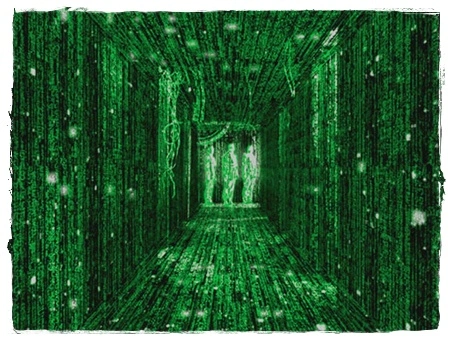
Most programmers young and old have seen the cyberpunk sci-fi film The Matrix. One of the most outstanding parts of the movie is the closing scene where Neo sees the Matrix when battling the Agents:

Neo Sees the Matrix

The visual effect with the code running along all the surfaces is iconic. Seems other people thought so too to the point that the effect has a name: Matrix Digital Rain.

Wouldn’t it be neat to create a terminal screensaver that mimicked the effect seen in the movie?

How to Make It Rain

Studying a few video compilations helps with understanding the details behind the scrolling effect:

{{< youtube E8y3eDUMb4Q >}}

Here are some features that pop out in the video:

  • The characters printed on the screen are a mix of Japanese kana and Latin letters/numeral characters.
  • Each column or stream has a fixed length with the first character in the stream having a bright white color.
  • Character streams spawn at random.
  • Once a stream of characters has begun, a new stream won’t begin on that column until all the previous characters have “fallen” off screen.

Fundamentally, a stream of characters scrolls down the screen. You can imagine the screen is a two dimensional matrix of characters. Each screensaver frame tick will scroll the screen down a single row such that the characters at the bottom row “fall off” the screen. The higher the framerate, the faster the characters fly down the screen.

Building a Scrolling Buffer

A handful of data structures implement the scrolling buffer effect. The first is the Char type:

struct Char {
    char c = '\0';
    bool first = false;
};

Char represents a single on-screen character. The only oddity here is the boolean first. You will see the purpose of the first field later.

The CharStream type represents the individual columns or streams of characters.

class CharStream {
   public:
    CharStream() = delete;

    CharStream(int capacity, int char_limit);
    ~CharStream() = default;
    CharStream(const CharStream&) = default;
    CharStream& operator=(const CharStream&) = default;
    CharStream(CharStream&&) = default;
    CharStream& operator=(CharStream&&) = default;
    void InsertChar(const Char& c);
    void RemoveChar();
    bool Empty() const { return (size_ <= 0); }
    int Size() const { return size_; }
    int Capacity() const { return static_cast<int>(chars_.capacity()); }
    int CharLimit() const { return char_limit_; }
    const Char& operator[](int i) const { return chars_[i]; }

   private:
    int size_;
    int char_limit_;
    bool limit_reached_;
    std::vector<Char> chars_;
};

CharStream is a fixed sized container type storing a limited number of non NULL Char objects. CharStream supports two primary operations: insert and remove.

InsertChar() inserts a Char at the beginning of the stream. The caller can only add up to char_limit_ characters to the stream. RemoveChar() removes the last Char in the stream by shifting all elements right a cell.

Below is a sequence of calls to a CharStream object demonstrating scrolling using the InsertChar() and RemoveChar() methods of the class:

CharStream stream(5, 3) -> [NULL, NULL, NULL, NULL, NULL]

stream.InsertChar('a')  -> [ 'a', NULL, NULL, NULL, NULL]
stream.RemoveChar()     -> [NULL,  'a', NULL, NULL, NULL]
stream.InsertChar('b')  -> [ 'b',  'a', NULL, NULL, NULL]
stream.RemoveChar()     -> [NULL,  'b',  'a', NULL, NULL]
stream.InsertChar('c')  -> [ 'c',  'b',  'a', NULL, NULL]

/* this insert is ignored because we have already reached the char limit of 3 */
stream.InsertChar('d') -> [ 'c',  'b',  'a', NULL, NULL]

stream.RemoveChar() -> [NULL,  'c', 'b',   'a', NULL]
stream.RemoveChar() -> [NULL, NULL, 'c',   'b',  'a']
stream.RemoveChar() -> [NULL, NULL, NULL,  'c',  'b']
stream.RemoveChar() -> [NULL, NULL, NULL, NULL,  'c']
stream.RemoveChar() -> [NULL, NULL, NULL, NULL, NULL]

Finally, ScreenBuffer implements the vertically scrolling buffer:

class ScreenBuffer {
   public:
    ScreenBuffer(int width, int height);
    ScreenBuffer() = delete;
    ~ScreenBuffer() = default;
    ScreenBuffer(const ScreenBuffer&) = default;
    ScreenBuffer& operator=(const ScreenBuffer&) = default;
    ScreenBuffer(ScreenBuffer&&) = default;
    ScreenBuffer& operator=(ScreenBuffer&&) = default;

    void Update();
    CharBuffer GetBuffer() const;

   private:
    std::size_t GetRandomNumInRange(int lower_bound, int upper_bound) const;
    char GetRandomBinDigit() const;
    void InsertChar(std::size_t stream_idx);
    void ScrollScreen();

    int width_;
    int height_;
    std::vector<CharStream> streams_;
};

At its core, ScreenBuffer is an array of CharStream objects where each CharStream represents a single screen column. The ScreenBuffer constructor ensures there are width many streams each with capacity and char limit of height. ScreenBuffer’s API updates the internal screen buffer and retrieves a read-only view of the buffer’s contents.

Update() is the heavy lifter which performs the following operations:

  1. Shifts all rows down by one. This deletes the bottom row and introduces a new, empty top row.
  2. If a column of characters hasn’t yet met its character limit, Update() will insert a character at the top of that column.
  3. Update() will select a random column index and will insert a character only if that column is empty.

With the data structures in place, all that’s left to do is render the ScreenBuffer’s contents using the ncurses API.

Rendering the Screensaver

The goal is to create a terminal screensaver. This limits your graphical library options. Good old ncurses will do.

For this project, binary digits are the only characters printed to the screen. No Japanese or Latin characters as in the original. This choice removed a lot of headaches while still keeping with the cyber theme of the original.

The ScreenSaver class renders the ScreenBuffer contents in a single ncurses window:

class ScreenSaver {
   public:
    ScreenSaver();
    ~ScreenSaver();
    ScreenSaver(const ScreenSaver&) = default;
    ScreenSaver& operator=(const ScreenSaver&) = default;
    ScreenSaver(ScreenSaver&&) = default;
    ScreenSaver& operator=(ScreenSaver&&) = default;

    void Draw();
    bool Quit() const { return (getch() != ERR); }

   private:
    enum Color {
        kWhite = 1,
        kGreen = 2,
    };

    ScreenBuffer buffer_;
};

The ScreenSaver API is simple: Draw() and Quit().

Quit() returns true if the User has pressed any key. It’s the mechanism by which the user can terminate the screensaver.

Draw() renders the ScreenBuffer’s contents in the window. Binary digits render in green with their dimness altered at random. The first character in each stream is the exception. If a Char’s first field is true, then that character is white and rendered in bold giving a visual cue as to where each stream starts.

The main screensaver loop ends up being simple:

int main() {
    const int kDefaultRefreshRateUsec = 75000;

    neo::ScreenSaver screensaver;
    while (!screensaver.Quit()) {
        screensaver.Draw();
        usleep(kDefaultRefreshRateUsec);
    }
    return 0;
}

The main loop continuously draws the screensaver with a delay between updates. If the user presses any key, the application exits.

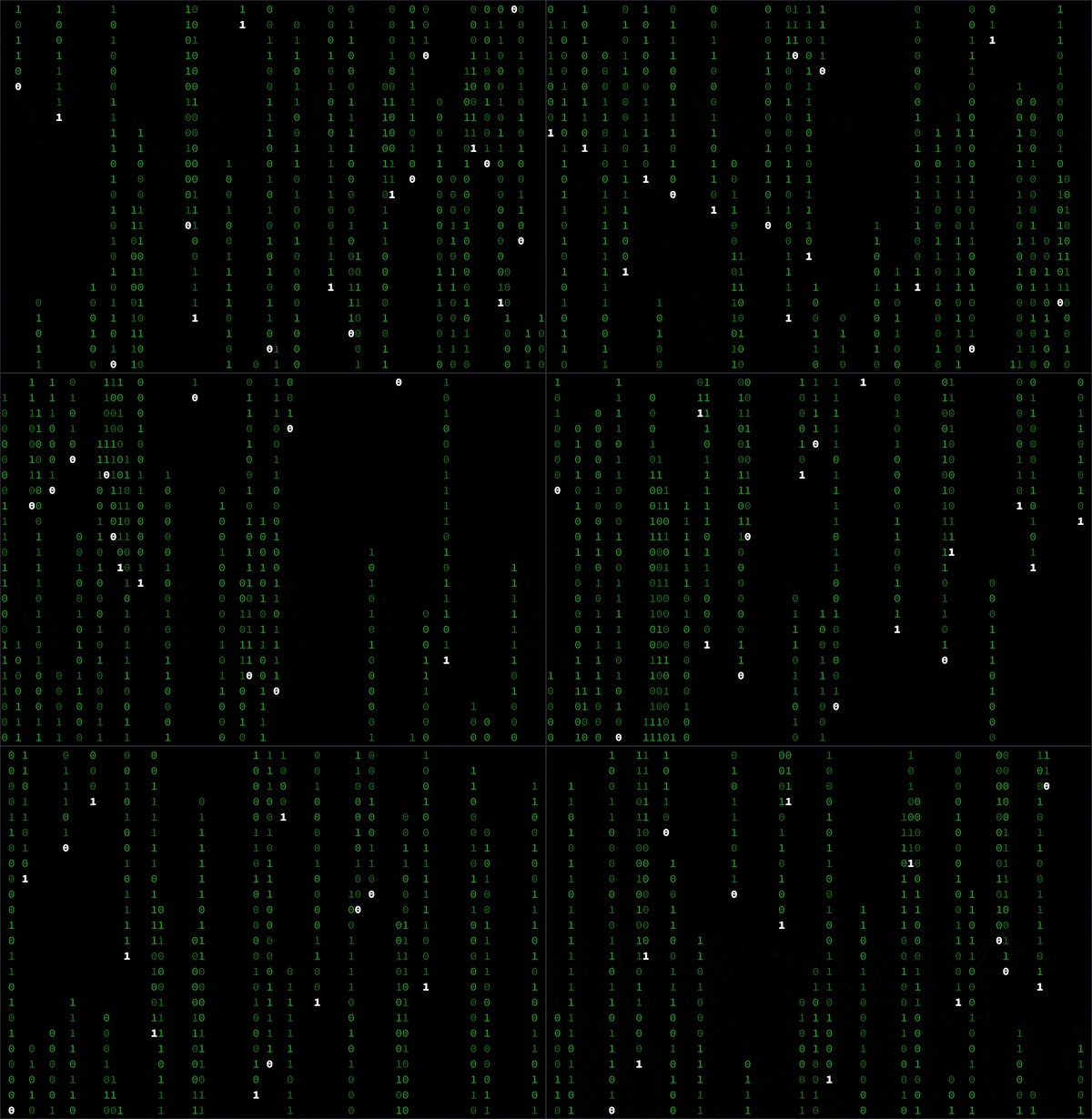
Here’s what the screensaver looks like in action:

Binary Rain

Conclusion

Making the neo screensaver had its challenges. In particular, this was one of those classic problems where if you have the right data structures its simple. Well sort of, implementing a tweaked scrolling buffer does take some thought. The setup presented here certainly cuts many corners with respect to efficiency. All that said, the screensaver has been fun to use at home and a great conversation piece amongst the Matrix nerds at work.

The complete project source with build instructions, usage, etc. is available on GitHub under neo.

read more →

A CLI Base Converter

When debugging an embedded system, it’s common to work with raw data requiring conversion between decimal, hexadecimal, binary, and sometimes octal number systems. The Python REPL and printf shell utility do the job but are tedious to use for the simple task of base conversion.

It would be nice to drop the overhead of format specifiers and fear of numerical limits. To ease the pain, I decided to write a command line utility that made conversion between positive binary, decimal, octal, and hexadecimal numbers of arbitrary size.

The Requirements

The use case is simple: take a positive integer in one base and convert it to the equivalent value in another base. That’s it. Support for negative values and floating point values is out of scope.

The program usage would look something like

dhb [OPTION]... SRC_BASE TGT_BASE NUM

where SRC_BASE/TGT_BASE are one of bin, dec, oct, or hex. NUM is some positive integer value.

Below are the requirements:

  1. Support conversions to/from binary, decimal, hexadecimal, and octal.
  2. Include an option for minimum output width.
  3. Include an option to group digits into segments of size N.
  4. Support arbitrarily large positive integers.

Requirement (1) is self explanatory. Requirement (2) means you can pad the output value with zeroes to achieve a minimum width. For example, pad the binary value 1111 to 8-bits leading to an output of 00001111. Requirement (3) is handy when you want to visualize binary or hex codes in groups of 4, 8, etc. digits. Taking the previous binary value of 00001111, maybe you want to group the bits into nibbles 0000 1111 or into 2 digits codes 00 00 11 11. Requirement (4) seems a bit extra but it has its value. Visualizing a large stream of hex values in binary is a common task. Exceeding the max integer limit for the system/program is also a common occurrence. This dhb tool should handle numbers outside the range of a uint64_t without breaking a sweat.

Lets look at how dhb meets each of these requirements starting with that bignum requirement.

Big, Huge Numbers

If you’re familiar with C++, you know the range of positive integers a program can work with is finite. There’s no standard “big number” library either.

Google search revealed a number of big number libraries. Most of the libraries are unmaintained, header-only libraries. The best option was the GNU MP Library (GMP). To quote the GMP homepage:

GMP is a free library for arbitrary precision arithmetic, operating on signed integers, rational numbers, and floating-point numbers. There is no practical limit to the precision except the ones implied by the available memory in the machine GMP runs on. GMP has a rich set of functions, and the functions have a regular interface.

GMP has a convenient C++ class based interface. The docs for how to use the C++ bindings and for GNU MP in general are solid. GMP is a perfect fit for this project.

Conversions

The only info needed to perform a conversion is the number, that number’s current base, and a target base. The conversion API accommodates this spec using one function and an enum:

enum NumSystem : int {
    kDec = 10,
    kHex = 16,
    kBin = 2,
    kOct = 8,
};

std::string ConvertBase(const std::string& num, const NumSystem src, const NumSystem target) {
    const mpz_class kTargetBase(static_cast<int>(target));
    const std::string kDigits("0123456789ABCDEF");

    std::string converted_num;
    mpz_class num_mp(num, static_cast<int>(src));
    while (num_mp) {
        mpz_class idx = num_mp % kTargetBase;
        converted_num += kDigits[idx.get_si()];
        num_mp /= kTargetBase;
    }
    std::reverse(converted_num.begin(), converted_num.end());

    return converted_num;
}

The algorithm for conversion is the usual change of base method which uses modulo and integer division to compute the digits of the output number one-by-one. The mpz_class is a GMP C++ wrapper class used to construct and manipulate big integral values. You can see mpz_class overloads the arithmetic operators such that the code doesn’t look much different than if one were to use the C/C++ built-in types.

One neat feature of GMP is the ability to construct an mpz_class object from a number represented as a string and its base. That feature makes implementation easier because you don’t have to massage the input into a format GMP understands. The constructor does throw std::invalid_arg if given an unsupported base argument. To avoid exceptions, the caller specifies the base using a NumSystem type which limits the caller to the bases known to the mpz_class constructor.

Formatting Output

Looking back at the requirements, there’s two formatting options to implement: minimum character width and digit grouping.

The minimum character width function was trivial to implement using a stringstream object in combination with stream modifiers:

std::string SetWidth(const std::string& num, int width) {
    if (width <= 0) {
        return num;
    }

    std::stringstream ss(num);
    ss << std::setfill('0') << std::setw(width) << num;

    return ss.str();
}

Not much to say here. The stream object will just slap zeroes onto the front of the number until it meets the width argument.

Segmenting the output’s digits into groups was a bit of a CS101 exercise:

std::string GroupDigits(const std::string& num, int grouping) {
    if ((grouping <= 0) || (grouping >= static_cast<int>(num.size()))) {
        return num;
    }

    std::stack<char> digits;
    for (const char& c : num) {
        digits.push(c);
    }

    std::string group;
    std::vector<std::string> groups;
    while (!digits.empty()) {
        group += digits.top();
        digits.pop();

        if (static_cast<int>(group.size()) == grouping) {
            std::reverse(group.begin(), group.end());
            groups.push_back(group);
            group = "";
        }
    }

    if (!group.empty()) {
        std::reverse(group.begin(), group.end());
        groups.push_back(group);
    }

    std::reverse(groups.begin(), groups.end());
    return std::accumulate(groups.begin(), groups.end(), std::string(),
                           [](const std::string& a, const std::string& b) {
                               return a + (a.empty() ? "" : " ") + b;
                           });
}

A stack processes the digits in the number from right to left. The algorithm pops characters off the stack into a group string. When that group string hits the grouping limit, it’s saved off in the groups vector and group is reset. Rinse and repeat.

Processing happens from right to left meaning there’s a reversal that needs to happen for each group string and for the entire groups vector. Without this reversal, the digits come out backwards in the output.

C++ doesn’t have a nice join() method like Python. Instead, you get to use the beautiful std::accumulate API to concatenate each string in groups using a single space as a separator. The concatenated string is the output of the function.

Testing the Implementation

At this point, you have a working conversion utility! The rest of the implementation focuses on command line argument parsing and input validation. You can check out the full source linked at the end of this article if you’re interested in those bits.

Lets test drive this tool:

dhb hex dec 0xDEADBEEF --> 3735928559
dhb dec bin 3735928559 --> 11011110101011011011111011101111
dhb dec oct 3735928559 --> 33653337357
dhb -g 4 dec hex 3735928559 --> DEAD BEEF
dhb -g 4 -w 12 dec hex 3735928559 --> 0000 DEAD BEEF

So far so good. Lets use a massive number like 2^64 * 12345 (AKA 227725055589944414699520). The tool should be able to handle that:

dhb --grouping 3 dec dec 227725055589944414699520 --> 227 725 055 589 944 414 699 520
dhb dec hex 227725055589944414699520 --> 30390000000000000000
dhb dec oct 227725055589944414699520 --> 60162000000000000000000000
dhb --grouping 8 hex bin --> 110000 00111001 00000000 00000000 00000000 00000000 00000000 00000000 00000000 00000000

Nice, looks to be working with big integers too.

The project includes a more complete suite of tests that exercises all the different conversion permutations.

Conclusion

The dhb utility has been of great use. The process of implementing the tool was relatively straightforward. I credit the simplicity to identifying early on the primary use cases and not tacking on too many bells and whistles along the way.

Note, this project has since been rewritten in Rust and renamed to nconv. The complete project source is available on GitHub under nconv. The Rust version of the project includes more testing but is otherwise a straight port of the C++.

read more →

Huffman Coding

Implementing a Huffman Tree is a fun afternoon project for anyone interested in learning about data compression. A Huffman Tree is a type of binary tree that sees use in the compression of an arbitrary data file. Developing a command line utility to compress/decompress a file using Huffman coding is a good CS101 challenge.

Breaking It Down Into Steps

This project starts where many do: Wikipedia. The Huffman Coding wiki article gives a nice breakdown with examples of the data structure and associated algorithms. In particular, the “Basic Technique” section covers the algorithms for compression and decompression. You need three key data structures to implement the big Compress() and Decompress() routines:

  1. A map mapping characters to their frequency in the input.
  2. A Huffman Tree used to generate an encoding map.
  3. An encodings map mapping characters to their binary code.

The next sections build up each structure and then discuss how they come together to implement Compress()/Decompress().

Constructing the Character Frequency Map

A key aspect of Huffman coding is the derivation of binary codes from the frequency of characters in the input file. The frequency of a character in the input drives the length of a character’s binary code. The higher the character frequency the shorter the binary code and vice versa.

So how do you track character frequency? A regular old map does the trick. The keys of the map are the characters in the input and the mapped to values are the character’s frequency. Below is a snippet of code showing how to construct a frequency map:

using CharFreqMap = std::map<char, uint32_t>;
CharFreqMap char_freqs_; /**< Map of character frequencies in the input. */

RetCode HuffmanCoding::CountCharFrequencies(const std::string& infile) {
    /* read the input file in kReadBuffSize sized chunks */
    std::ifstream infile_stream(infile, std::ios::binary);
    while (infile_stream) {
        infile_stream.read(read_buffer_.data(), read_buffer_.size());
        for (std::streamsize i = 0; i < infile_stream.gcount(); ++i) {
            char_freqs_[read_buffer_[i]]++; /* up the char's frequency */
        }
    }
    return (char_freqs_.empty()) ? RetCode::kEmptyFile : RetCode::kSuccess;
}

The code reads character data into the read_buffer_ buffer in 1 kilobyte chunks. The char_freqs_ map tracks the frequency of each character.

Growing a Huffman Tree

You now have a map of character frequencies. How do you use this frequency map to generate binary codes? There’s an intermediate step. You need to represent your character frequencies in a way that you can later use to generate optimal codes. This is where the infamous Huffman Tree comes into play.

A Huffman Tree is a binary tree. The nodes of a Huffman Tree often have a structure like this:

struct HuffmanNode {
    int character;       /**< Character or kInternalNode value. */
    uint32_t count;      /**< Character frequency. */
    HuffmanNodePtr zero; /**< Huffman tree left subtree. */
    HuffmanNodePtr one;  /**< Huffman tree right subtree. */
};

Here’s a picture of a Huffman Tree for the input text aaaaabbc:

                                   ┌───────────────────────────┐
                                   │          Node 1           │
                                   ├───────────────────────────┤
                                   │character = INTERNAL_MARKER│
                                   ├───────────────────────────┤
                                   │count = 8                  │
                                   └─────────────┬─────────────┘

                             ┌─────────0─────────┴───────1──────┐
                             │                                  │
                ┌────────────▼──────────────┐       ┌───────────▼───────────────┐
                │          Node 2           │       │          Node 3           │
                ├───────────────────────────┤       ├───────────────────────────┤
                │character = INTERNAL_MARKER│       │character = 'a'            │
                ├───────────────────────────┤       ├───────────────────────────┤
                │count = 3                  │       │count = 5                  │
                └─────────────┬─────────────┘       └───────────────────────────┘

             ┌────────0───────┴───────1───────┐
             │                                │
┌────────────▼──────────────┐    ┌────────────▼──────────────┐
│          Node 4           │    │          Node 5           │
├───────────────────────────┤    ├───────────────────────────┤
│character = 'c'            │    │character = 'b'            │
├───────────────────────────┤    ├───────────────────────────┤
│count = 1                  │    │count = 2                  │
└───────────────────────────┘    └───────────────────────────┘

There are two types of nodes in the tree: internal nodes and leaf nodes. The leaf nodes of a Huffman Tree contain an input character and its frequency (denoted as count in the image). The internal nodes of a Huffman Tree often replace the character with some special marker value and contain a count value equal to the sum of the count values of its subtrees. By convention, the edge to the left subtree has a label of zero and the edge to the right subtree has a label of one.

Notice how the root to leaf path for the highest frequency character, a, is shorter than the root to leaf paths for the lower frequency chars. This is no coincidence. You traverse a Huffman Tree such that you obtain character to binary string mappings where the most frequent characters have the most compact representation.

So how do you build the tree from the frequency map? The wiki article provides an algorithm for constructing an optimal Huffman Tree:

  1. Start with as many leaves as there are symbols.
  2. Enqueue all leaf nodes into the first queue (by probability in increasing order so that the least likely item is in the head of the queue).
  3. While there is more than one node in the queues:
    • Dequeue the two nodes with the lowest weight by examining the fronts of both queues.
    • Create a new internal node, with the two just-removed nodes as children (either node can be either child) and the sum of their weights as the new weight.
    • Enqueue the new node into the rear of the second queue.
  4. The remaining node is the root node; the tree has now been generated.

Below is a C++ implementation of the algorithm description:

using HuffmanNodePtr = std::shared_ptr<HuffmanNode>;

void HuffmanCoding::BuildEncodingTree() {
    auto HuffmanNodePtrGreater = [](const HuffmanNodePtr a,
                                    const HuffmanNodePtr b) {
        return (a->count > b->count);
    };
    std::priority_queue<HuffmanNodePtr, std::vector<HuffmanNodePtr>,
                        decltype(HuffmanNodePtrGreater)>
        encoding_queue;

    /* load the initial nodes with their chars and freqs */
    for (const auto& [character, frequency] : char_freqs_) {
        encoding_queue.push(
            std::make_shared<HuffmanNode>(character, frequency));
    }

    /* follow the algorithm described in
     * https://en.wikipedia.org/wiki/Huffman_coding under the "Compression"
     * section */
    while (encoding_queue.size() != 1) {
        HuffmanNodePtr first = encoding_queue.top();
        encoding_queue.pop();
        HuffmanNodePtr second = encoding_queue.top();
        encoding_queue.pop();

        HuffmanNodePtr new_node = std::make_shared<HuffmanNode>(
            kInternalNode, first->count + second->count, first, second);

        encoding_queue.push(new_node);
    }
    encoding_root_ = encoding_queue.top(); /* save off the root of the tree */
}

When BuildEncodingTree() terminates, encoding_root_ will point to the root node of the Huffman Tree.

Building a Codebook

It’s the moment you’ve been waiting for: code generation. You probably already guessed how this works. To generate a character’s code, all you need to do is traverse the Huffman Tree. As you walk down from the root to each leaf, you bookkeep the path taken using 0’s to indicate left subtree traversals and 1’s for the right subtree traversals. When you hit a leaf node, you save off the node’s character value and the bit string generated up to that node.

Here’s a snippet showing how to recursively construct character encodings:

using EncodingMap = std::map<char, std::string>;
EncodingMap encodings_; /**< Map of character to binary string encodings. */

void HuffmanCoding::BuildEncodingMap(HuffmanNodePtr root,
                                     std::string encoding) {
    if (root->character != kInternalNode) { /* reached a leaf node */
        encodings_[static_cast<char>(root->character)] = encoding;
        return;
    }
    BuildEncodingMap(root->zero, encoding + "0"); /* recurse into ltree */
    BuildEncodingMap(root->one, encoding + "1");  /* recurse into rtree */
}

At the end of this routine, encodings_ will contain a mapping of each character in the input to a binary string. Using the example text aaaaabbc given in the previous section, the encodings_ map would look like

CharacterEncoding
a1
b01
c10

The original text required one byte per character or 8 bytes of storage. Using this codebook, you could store the text string using the code 11111010110. This would require only two bytes to store the same information. Why two bytes? Because you can only write in units of bytes to an output file meaning you have to pad the bit string with 5 zeroes on the right (for example, 11111010 110 -> 11111010 11000000).

Compression

With codebook in hand, compression boils down to converting an input stream into a coded bit stream. Then, write out the contents of the bit stream byte-by-byte to an output file.

Here is an implementation of the Compress() routine:

RetCode HuffmanCoding::Compress(const std::string& uncompressed_filepath,
                                const std::string& compressed_filepath) {
    /* verify uncompressed_filepath points to an existing file */
    std::filesystem::path uncompressed_path(uncompressed_filepath);
    if (!std::filesystem::exists(uncompressed_filepath)) {
        return RetCode::kFileDoesNotExist;
    }

    /* scan the uncompressed file once to compute char frequencies */
    RetCode retcode = CountCharFrequencies(uncompressed_filepath);
    if (RetCode::kSuccess != retcode) {
        return retcode;
    }

    BuildEncodingTree();                  /* construct the huffman code tree */
    BuildEncodingMap(encoding_root_, ""); /* construct char to bit string map */
    Encode(uncompressed_filepath, compressed_filepath); /* compress the data */

    return retcode;
}

You can see that Compress() just does some file checks and then builds up the data structures previously discussed. Encode() is where the actual translation happens. The code for Encode() is a bit ugly:

void HuffmanCoding::Encode(const std::string& infile,
                           const std::string& outfile) {
    /* controls for writing compressed data byte by byte */
    const int kBitsPerByte = 8;
    uint8_t currbyte = 0;
    int bitcount = 0;

    std::ofstream outfile_stream(outfile, std::ios::out | std::ios::binary);
    WriteHeader(outfile_stream); /* write the compressed files' header first */

    std::ifstream infile_stream(infile, std::ios::in);
    while (infile_stream) {
        /* read uncompressed data */
        infile_stream.read(read_buffer_.data(), read_buffer_.size());

        /* encode the chars in the buffer */
        for (std::streamsize i = 0; i < infile_stream.gcount(); ++i) {
            /* since the smallest unit we can write to a file is a byte not a
             * bit, the code below constructs a byte from the bits in an
             * encoding and then writes the byte to the output file */
            for (const char& bit : encodings_.at(read_buffer_[i])) {
                uint8_t ibit = (bit == '1') ? 1 : 0;
                currbyte = (currbyte << 1) | ibit;
                bitcount++;
                if (bitcount == kBitsPerByte) {
                    outfile_stream.write(reinterpret_cast<char*>(&currbyte),
                                         sizeof(currbyte));
                    currbyte = 0;
                    bitcount = 0;
                }
            }
        }
    }

    if (bitcount) { /* the very last character didn't land on the byte boundary
                       so we need to pad it with zeroes before writing it out to
                       file */
        while (bitcount != kBitsPerByte) {
            currbyte <<= 1;
            bitcount++;
        }
        outfile_stream.write(reinterpret_cast<char*>(&currbyte),
                             sizeof(currbyte));
    }
}

Encode() reads the input file in 1kb chunks. The encodings_ codebook makes it possible to find each character’s binary code. You iterate each binary code bit-by-bit appending each bit to the variable currbyte. When currbyte’s bitcount hits 8, you write currbyte out to file. This process repeats until you have processed all characters in the input. The if (bitcount) clause at the end handles the edge case previously discussed where you need to append a couple of zeroes to a binary code to make it a complete byte before writing to the file.

You might have noticed a call to WriteHeader(). You’ll see the purpose of WriteHeader() in the next section.

Decompression

Assuming you have the Huffman Tree used to compress a file available, decompressing the contents of the file requires only a tree traversal. Imagine the compressed file is a bit stream. You can navigate the tree from the root using the current bit in the stream to guide whether you step into the left subtree or right subtree. When you encounter a leaf node, write the character of that node to an output file and then reset to the root of the tree.

As always, the devils in the details. For this tree traversal to work, you need to know the following bits of information:

  • How to reconstruct the Huffman Tree.
  • How many characters were in original input file.

Two Birds With One Stone

An easy way of reconstructing the tree is to write out the character frequency table to the beginning of the file in a header section. Writing the whole table isn’t particularly efficient for small input files given that the header will be significantly larger than the compressed data. However, as the input grows, the overhead of the header becomes negligible.

Included in the header is a magic number. That magic number forms the first few bytes of the compressed file and helps identify a file as a Huffman coded file.

Here’s how that header might look like in memory:

Huffman Header

Below is the header generation code in all its glory:

void HuffmanCoding::WriteHeader(std::ofstream& os) const {
    os.write(reinterpret_cast<const char*>(&kHuffmanFmtIdentifier),
             sizeof(kHuffmanFmtIdentifier));

    std::size_t num_chars = char_freqs_.size();
    os.write(reinterpret_cast<char*>(&num_chars), sizeof(num_chars));

    for (const auto& [character, frequency] : char_freqs_) {
        os.write(&character, sizeof(character));
        os.write(reinterpret_cast<const char*>(&frequency), sizeof(frequency));
    }
}

WriteHeader() solves the problems encountered earlier: how to reconstruct the tree and how many characters were in the uncompressed file. Using the frequency table parsed from a compressed file’s header, you can run the BuildEncodingTree() routine just as before. A quick sum of the frequencies in the char_freqs_ maps reveals how many characters were in the original input.

Decoding Data

You can decompose the Decompression() routine into three separate parts:

  1. Reading the header.
  2. Building the encoding tree.
  3. Decoding the input bit stream.

You already have a routine to write the header. The function that reads the header is similar. Just replace stream writes with reads. Once you read the header, building the encoding tree requires calling BuildEncodingTree(). Decoding the bit stream is the only new thing here.

Here’s the code that implements the concept:

void HuffmanCoding::DecodeStream(const std::vector<bool>& bitstream,
                                 std::ofstream& os) {
    /* take a tally of how many chars we need to decode */
    uint32_t num_chars = 0;
    for (const auto& kv : char_freqs_) {
        num_chars += kv.second;
    }

    /* repeatedly traverse the huffman tree decoding characters along the way */
    uint32_t num_chars_decoded = 0;
    HuffmanNodePtr node = encoding_root_;
    std::size_t i = 0;
    while ((i < bitstream.size()) && (num_chars_decoded != num_chars)) {
        node = (bitstream[i]) ? node->one : node->zero;

        if (!node->zero && !node->one) { /* reached a leaf node */
            os << static_cast<char>(node->character);
            node = encoding_root_;
            num_chars_decoded++;
        }
        i++;
    }
}

One weak aspect of this code is that DecodeStream() expects the entire input bit stream at once. That is, all bits (represented as bool types) are in memory and buffered. If the file is large enough, the bitstream vector may well not fit in memory. For this project, it’s reasonable to keep it simple and not worry about multi gigabyte files. A better approach would be to read the data, perhaps in page sized chunks, and create a parser object that tracks where in the decoding process it is.

Similar to Compress(), the Decompress() routine is a wrapper around the Decode() routine:

RetCode HuffmanCoding::Decode(const std::string& infile,
                              const std::string& outfile) {
    std::ifstream infile_stream(infile, std::ios::in | std::ios::binary);
    RetCode retcode = ReadHeader(infile_stream); /* read in char frequencies */
    if (RetCode::kSuccess != retcode) {          /* invalid header */
        return retcode;
    }

    BuildEncodingTree(); /* construct the encoding tree */

    /* build up a bit vector from the compressed file's binary content */
    const int kNumBitsInByte = 8;
    std::vector<bool> bitstream;
    while (infile_stream) {
        infile_stream.read(read_buffer_.data(), read_buffer_.size());
        for (std::streamsize i = 0; i < infile_stream.gcount(); ++i) {
            for (int j = 0; j < kNumBitsInByte; ++j) {
                uint8_t mask = 1 << (kNumBitsInByte - j - 1);
                bitstream.push_back(read_buffer_[i] & mask);
            }
        }
    }

    /* reconstruct the message by traversing the huffman tree */
    std::ofstream outfile_stream(outfile);
    DecodeStream(bitstream, outfile_stream);

    return retcode;
}

RetCode HuffmanCoding::Decompress(const std::string& compressed_filepath,
                                  const std::string& uncompressed_filepath) {
    /* verify compressed_filepath points to an existing file */
    std::filesystem::path compressed_path(compressed_filepath);
    if (!std::filesystem::exists(compressed_filepath)) {
        return RetCode::kFileDoesNotExist;
    }

    return Decode(compressed_filepath, uncompressed_filepath);
}

Conclusion

Putting it all together, you have a utility capable of compressing and decompressing any image, text, executable, etc. using Huffman coding. The implementation isn’t the most robust or efficient with regards to space/time. The header could be significantly smaller. You probably shouldn’t pass in any files that don’t fit in memory. That said, the core concepts are there. Playing around with the tool, you’ll find some files compress down to 50% of their original size!

Note, this project has since been rewritten in Rust. The complete project source is available on GitHub under huffman. The Rust version of the project includes more testing, better error handling, and buffered IO.

read more →

Digital Image Steganography

There’s a neat Computerphile video discussing the topic of steganography. In the video, Mike Pound talks about a technique for steganography on digital images: least significant bit substitution (LSBS). The effectiveness of LSBS in concealing a secret image is surprising. This article puts least significant bit substitution to use in a command line tool for embedding one image within another.

A Little Background on Digital Images

You don’t need fancy image manipulation techniques to make this steganography tool work. That said, you do need to know a little bit about how the machine represents a digital image.

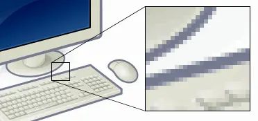
A digital image can contain thousands of pixels. Below is an image where the enhanced portion shows the pixels rendered as small squares.

Pixels

3 to 4 channels describe each pixel in an image. There’s the classic red, green, and blue (RGB) pixel and the cyan, magenta, yellow, and black (CYMK) pixel. This articles focuses on three channel or RGB pixels.

Each channel of an RGB pixel specifies the intensity of the color using an 8-bit value. Combining the three channels, you’re able to represent 2^24 or well over 16 million different colors. Often, hexadecimal numbers describe each byte of an RGB color pixel as shown in the table below.

RGB Color Palette

A digital image is a two dimensional matrix of pixel values. The steganography algorithm discussed here will encode the pixel data of one secret image in the pixel data of another cover image using a reversible process.

Least Significant Bit Substitution

LSB substitution works on the principal that the most significant bits (MSBs) of a number have a much larger impact on the numerical value than the least significant bits (LSBs). As an example, imagine you had the 16-bit value 1101010101001000 which in decimal is 54600. If you flipped the MSB, the binary number would be 0101010101001000 or 21832 decimal. That’s approximately a 60% difference from changing a single bit! Now say you went crazy and flipped the lowest 8 bits producing 1101010110110111 or 54711. Despite flipping 7 more bits, you only see an approximately 0.002% difference in the numerical value.

So how does this apply to image steganography? You can hide the MSBs of your secret image’s pixels in the LSBs of your cover image. You apply this process to each color channel in the pixel. If the cover image is a noisy one, then the change will be unnoticeable to the human eye. You simply reverse the process to recreate the secret image: make the LSBs of the merged image the MSBs of the new unmerged image with the lower bits zeroed out. You lose information in this merge/unmerge process. The loss is sometimes obvious in the unmerged image as you will see in a later example.

Here’s an example using the 4 least significant bits of each color channel.

Suppose you had a cover image pixel with the following RGB values represented in hexadecimal:

ChannelValue
R0xFA
G0x1B
B0xC9

Your corresponding secret pixel might look something like:

ChannelValue
R0x12
G0x78
B0xFF

The merge operation has you take the most significant hex digit (that is, 4-bits) of the secret pixel and place them as the least significant hex digit of the cover image (highlighted below). The merged pixel would then look like:

ChannelValue
R0xF1
G0x17
B0xCF

To retrieve the secret pixel from a merge pixel, you take the least significant 4 bits of the merged pixel and concatenate it with zeroes on the right:

ChannelValue
R0x10
G0x70
B0xF0

How many bits should you use to conceal your image? That depends on the cover and secret image. 4-bits is a rough upper limit. Using more than 4-bits often leads to artifacts in the merged image. The examples and code presented in this article use the 4 LSBs of each channel. It’s straightforward to modify the code to work with different LSB counts.

Making It Happen

The idea is to have a command line tool that could merge and unmerge two images. Program usage looks something like:

$ steganography merge cover.jpg secret.jpg out.png
...
$ steganography unmerge out.png secret.jpg

If you ignore all the argument processing and error checking code, the program boils down to implementing two functions: Merge() and Unmerge().

Merging

Below is a snippet showing the interesting bits of the merge implementation:

static boost::gil::rgb8_pixel_t MergePixels(
    const boost::gil::rgb8_pixel_t& cover_pix,
    const boost::gil::rgb8_pixel_t& secret_pix) {
    const int kHighNibble = 0xF0;
    boost::gil::rgb8_pixel_t merged_pix(0, 0, 0);
    for (int i = 0; i < 3; ++i) {
        merged_pix[i] =
            (cover_pix[i] & kHighNibble) | ((secret_pix[i] & kHighNibble) >> 4);
    }
    return merged_pix;
}

RetCode Merge(const std::string& cover, const std::string& secret,
              const std::string& outfile) {
    ...

    /* load images into GIL image type */
    boost::gil::rgb8_image_t cover_img(ReadImage(cover, cover_img_t));
    boost::gil::rgb8_image_t secret_img(ReadImage(secret, secret_img_t));
    boost::gil::rgb8_image_t output_img = cover_img;

    ...

    /* merge the secret image's pixels into the output image */
    const boost::gil::rgb8_pixel_t kBlackPixel(0, 0, 0);
    auto secret_view = boost::gil::const_view(secret_img);
    auto output_view = boost::gil::view(output_img);
    for (int row = 0; row < output_view.height(); ++row) {
        for (int col = 0; col < output_view.width(); ++col) {
            if ((row >= secret_img.height()) || (col >= secret_img.width())) {
                output_view(col, row) =
                    MergePixels(output_view(col, row), kBlackPixel);
            } else {
                output_view(col, row) =
                    MergePixels(output_view(col, row), secret_view(col, row));
            }
        }
    }

    ...
}

You can see the Merge() function iterates over the output_view. output_view is a mutable Boost GIL image view into a deep copy of cover_img. For each pixel in output_view, you call MergePixels() which applies the 4-bit merge operation previously described to each of the three color channels.

Since your secret image may be smaller in dimension than your cover image, whenever a pixel in output_view is out of range of secret_view, you merge output_view’s pixel with a black pixel. This means that when the secret image’s dimensions are less than that of the cover image, the image that’s later unmerged will have a black border.

Below are three images showing the output of a merge command. From left to right you have the cover image, secret image, and merged image. You can view the actual image files here.

Cover Image
Secret Image
Merged Image

Unmerging

Here are the critical parts of the unmerge implementation:

static boost::gil::rgb8_pixel_t UnmergePixels(
    const boost::gil::rgb8_pixel_t& pixel) {
    const int kLowNibble = 0x0F;
    boost::gil::rgb8_pixel_t unmerged_pix(0, 0, 0);
    for (int i = 0; i < 3; ++i) {
        unmerged_pix[i] = (pixel[i] & kLowNibble) << 4;
    }
    return unmerged_pix;
}

RetCode Unmerge(const std::string& secret, const std::string& outfile) {
    ...

    /* load images into GIL image type */
    boost::gil::rgb8_image_t secret_img(ReadImage(secret, secret_img_t));
    boost::gil::rgb8_image_t output_img = secret_img;

    /* extract the hidden image into the output image */
    auto secret_view = boost::gil::const_view(secret_img);
    auto output_view = boost::gil::view(output_img);
    for (int row = 0; row < output_view.height(); ++row) {
        for (int col = 0; col < output_view.width(); ++col) {
            output_view(col, row) = UnmergePixels(secret_view(col, row));
        }
    }

    ...
}

Not too much to harp on here. This is the inverse of the Merge() function. The key is that you know how many bits formed the secret during merging. Now you can pop the proper bits from the LSBs of the merged image to the MSBs of the output image.

Below is the original secret image on the left and the unmerged image on the right. Notice the loss in quality in the unmerged image. This happens because you lost the 4 LSBs of each pixels’ color channels when performing the merge operation.

Secret Image
Unmerged Image

A Note on Image Formats

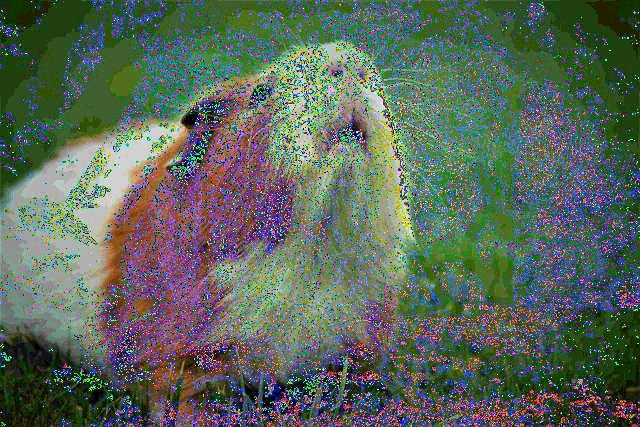
There’s a fun file format related bug worth discussing. It turns out some image formats are lossy. What this means is that when you format your image data using one of these lossy formats, you lose or alter pixel data. This is bad news for this naive image steganography tool. Just take a look at what happens to the poor guinea pig after a merge to JPEG:

Mangled Guinea Pig

The steganography tool presented here supports just two image formats: JPEG and PNG. JPEG is a lossy format. PNG is a lossless format. The easy solution is to require that the output of a merge command always be a PNG. This implies the input to an unmerge command is always a PNG. The output of an unmerge command can be either format.

Conclusion

The least significant bit substitution method proved simple to implement and doesn’t disappoint in its effectiveness in secretly embedding one image within another. Interested in a more serious steganography tool? Highly recommend checking out a free and open source tool such as steghide.

Note, this project has since been rewritten in Rust and renamed to steg. The complete project source is available on GitHub under steg. The Rust version of the project includes more testing, support for additional image formats, and the ability to chose the number of bits to use for the merge/unmerge operation.

read more →

Snake in the Terminal

Are you a text user interface enjoyer? Have you always wondered how difficult is it to write an ncurses UI? What better way to find out than to write a program of your own that explores ncurses’ API. Of course, you have to keep it interesting. Why not implement a scaled down version of a retro arcade game: snake.

The Rules of Snake

Step one of this project is to look up what the rules for a game of snake are. Specifically, what does the play “arena” look like, how do you win, and how do you lose?

The play arena is simple: it’s a 2D rectangle divvied up into 1x1 tiles. The arena is static meaning once the game starts the dimensions of the play area don’t change. There are two objects in the arena at any given time: a target and the snake. The target consumes a single tile and spawns randomly on any tile except those occupied by the snake. The snake is one or more adjacent tiles with no more than two tiles being adjacent to one another. Below is a target (red diamond) and snake made up of 13 tiles.
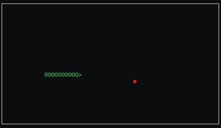
Snake Objects

To win the game, the snake must cover all tiles that make up the play arena. Each time the snake’s head intersects or “eats” a target, the snake grows in length by a single tile. The player controls the snake and can only move it up, down, left, or right. If the player manages to cover the whole arena in snake tiles, they win.

There’s two ways to lose:

  1. The snake goes out of the play arena bounds.
  2. The snake tries to eat itself.

Targets just keep spawning on open tiles until the snake gets itself in a losing situation or wins by taking over all the tiles. That’s it! That’s all there is to this game.

Implementing the Game

The key goal here is to learn about the ncurses library not necessarily implement the most theoretically space/time efficient version of snake. With that in mind, you can take the stupid simple approach to implementing the game.

The core data structure is the Tile type:

enum class Direction {
    kUp,
    kDown,
    kLeft,
    kRight,
    kNone,
};

struct Tile {
    int row = 0;
    int col = 0;
    Direction direction = Direction::kNone;

    friend bool operator==(const Tile& a, const Tile& b) {
        return ((a.row == b.row) && (a.col == b.col));
    }
};

The snake itself is a 1D vector of Tile objects. Similarly, a 1D vector of Tile objects represents all the possible locations a target can spawn:

using Snake = std::vector<Tile>;
using Targets = std::vector<Tile>;
Snake snake_;
Target targets_;

With these simple data structures, implementing the core logic of the game is relatively straightforward. These next few sections will cover the core algorithms and their implementations.

Initialization

Initializing the game involves two key steps: generating all possible target locations and spawning the snake. You can bundle both these steps into a single Reset() function that resets the game to its initial state.

Generating all possible targets requires creating a Tile object for each 1x1 tile on the screen. The added twist is that the targets_ vector must get shuffled. The reasoning behind the shuffling is to make the selection of a random target tile easier in the main game loop.

The snake itself initially consists of one Tile located in the center of the screen with a random direction. One thing to be wary of is that you don’t want the initial target tile intersecting the snake. Hence the while loop that updates the current target tile index if it overlaps with the snake’s initial spawn Tile:

void SnakeGame::SpawnSnake() {
    /* create a random shuffle of the possible directions the snake can go */
    std::vector<Direction> directions = {Direction::kUp, Direction::kDown,
                                         Direction::kLeft, Direction::kRight};
    auto rd = std::random_device{};
    auto rng = std::default_random_engine{rd()};
    std::shuffle(directions.begin(), directions.end(), rng);

    /* spawn the snake head in the center of the screen with a random direction
     */
    snake_.push_back({.row = screen_dim_.height / 2,
                      .col = screen_dim_.width / 2,
                      .direction = directions[0]});
}

void SnakeGame::Reset() {
    game_over_ = false;
    score_ = 0;

    /* generate a randomly shuffled vector of potential target locations */
    targets_.clear();
    for (int i = border_; i < (screen_dim_.height - border_); ++i) {
        for (int j = border_; j < (screen_dim_.width - border_); ++j) {
            targets_.push_back(
                {.row = i, .col = j, .direction = Direction::kNone});
        }
    }
    auto rd = std::random_device{};
    auto rng = std::default_random_engine{rd()};
    std::shuffle(targets_.begin(), targets_.end(), rng);
    curr_target_ = 0;

    /* respawn the snake */
    snake_.clear();
    SpawnSnake();

    /* ensure the target does not overlap the snake head */
    while (targets_[curr_target_] == snake_.front()) {
        curr_target_ = (curr_target_ + 1) % static_cast<int>(targets_.size());
    }
}

Moving the Snake

Moving the snake is tricky. The snake head Tile updates its row or col depending on the value of its direction field. All other Tile objects assume the position and values of the Tile that precedes it.

void SnakeGame::MoveSnake(const Direction& new_direction) {
    /* shift all but the head tiles into their predecessor's position */
    Snake tmp = snake_;
    for (std::size_t i = 1; i < snake_.size(); ++i) {
        snake_[i] = tmp[i - 1];
    }

    /* walk the head forward in whatever direction it's facing */
    Tile& head = snake_.front();
    head.direction = new_direction;
    switch (snake_.front().direction) {
        case Direction::kUp:
            head.row--;
            break;
        case Direction::kDown:
            head.row++;
            break;
        case Direction::kLeft:
            head.col--;
            break;
        case Direction::kRight:
            head.col++;
            break;
        case Direction::kNone:
            break;
    }
}

You’ll notice there’s a copy of the entire snake_ vector into a temporary vector, tmp. There’s tricks to avoid this overhead, but they’re all overkill considering how lightweight the game objects are. This pattern of going with the less computationally efficient but more obvious implementation is one you’ll see repeating here.

Snake Extension

Growing the snake is funky as well. You technically want to extend from the tail. The question is, in which direction? One approach is to add a new tile just one tile opposite the current tail.

void SnakeGame::ExtendSnake() {
    Tile new_snake_tile = snake_.back();

    /* the new tile's location is the current snake tail's location shifted
     * opposite the snake tail's direction */
    switch (new_snake_tile.direction) {
        case Direction::kUp:
            new_snake_tile.row++;
            break;
        case Direction::kDown:
            new_snake_tile.row--;
            break;
        case Direction::kLeft:
            new_snake_tile.col++;
            break;
        case Direction::kRight:
            new_snake_tile.col--;
            break;
        case Direction::kNone:
            break;
    }
    snake_.push_back(new_snake_tile);
}

Winning

To win, the snake must cover every possible arena tile. Since the targets_ vector has every possible arena Tile contained within it, checking for a win means checking whether the snake_ vector equals the targets_ vector.

bool SnakeGame::SnakeWins() const {
    /* check whether the snake is occupying every possible target location */
    for (const Tile& target_tile : targets_) {
        bool found = false;
        for (const Tile& snake_tile : snake_) {
            if (snake_tile == target_tile) {
                found = true;
                break;
            }
        }
        if (!found) { /* looks like there's at least one open target location */
            return false;
        }
    }
    return true;
}

This good old O(N2)\mathcal{O}(N^2) time complexity double nested loop does the trick.

Losing

Another O(N2)\mathcal{O}(N^2) algorithm determines whether a player lost. In this case, the majority of the time goes into checking whether the snake is overlapping with itself.

bool SnakeGame::IsGameOver() const {
    /* check if the snake overlaps itself at any tile */
    for (std::size_t i = 0; i < snake_.size(); ++i) {
        for (std::size_t j = i + 1; j < snake_.size(); ++j) {
            if (snake_[i] == snake_[j]) {
                return true;
            }
        }
    }

    /* verify the head snake tile is in bounds */
    bool is_in_row_bounds =
        (snake_.front().row >= border_) &&
        (snake_.front().row < (screen_dim_.height - border_));
    bool is_in_col_bounds =
        (snake_.front().col >= border_) &&
        (snake_.front().col < (screen_dim_.width - border_));

    return (!is_in_row_bounds || !is_in_col_bounds);
}

You might have noticed a border_ value in the bounds checks. The game arena can optionally include a border. With the border included, the snake can’t make contact with the border else the game is over. Hence why the border_ variable is part of the bounds check logic.

The Game Tick

This version of snake operates using game ticks. On a single game tick the snake will move and logic will execute to determine whether the player has won, lost, ate a target, etc. The Tick() method only accepts a Direction value indicating the direction the player commanded the snake to move.

void SnakeGame::Tick(const Direction& new_direction) {
    MoveSnake(new_direction);

    if (IsGameOver()) { /* do nothing if the game has already ended */
        game_over_ = true;
        return;
    }

    /* looks like the snake ate its target */
    if (snake_[0] == targets_[curr_target_]) {
        score_ += kScoreIncrement;

        ExtendSnake();

        if (SnakeWins()) {
            game_over_ = true;
            return;
        }

        /* search for the next target tile that is not occupied by the snake */
        while (std::find(snake_.begin(), snake_.end(),
                         targets_[curr_target_]) != snake_.end()) {
            curr_target_ =
                (curr_target_ + 1) % static_cast<int>(targets_.size());
        }
    }
}

User Interface Design with ncurses

With the game logic and state wrapped in a neat class, it’s time to write the UI. You need to see what API calls ncurses provides and examples of how folks organize their ncurses programs. There’s an aptly named site that does all those things: NCURSES Programming HOWTO. The articles provides an API walk through with clear examples you can test and mod. The site also has sections explaining the use of related ncurses libraries for menus, forms, and more.

Ncurses provides a C API that like most C APIs is unforgiving when you get it wrong. RTFM applies when using just about any function in this library. To keep things manageable, split the game into three primary views: start screen, game screen, game over screen.

Start Screen

A simple game should have a simple start menu. An ASCII art title banner followed by a menu from which the player selects one of three difficulty modes seems fitting. Ncurses can certainly handle drawing banner and prompt text. However, to implement the mode menu, you should use menu library. The menu library extends ncurses and provides wrapper functions that simplify menu creation.

Here’s the code that displays the game start screen:

GameMode PromptForGameMode() {
    clear();

    const std::vector<std::string> kTitleBanner = {
        " _____  _   _   ___   _   __ _____ ",
        "/  ___|| \\ | | / _ \\ | | / /|  ___|",
        "\\ `--. |  \\| |/ /_\\ \\| |/ / | |__  ",
        " `--. \\| . ` ||  _  ||    \\ |  __| ",
        "/\\__/ /| |\\  || | | || |\\  \\| |___ ",
        "\\____/ \\_| \\_/\\_| |_/\\_| \\_/\\____/ ",

    };

    /* display the title banner */
    int row = 0;
    int col = 0;
    getmaxyx(stdscr, row, col);
    (void)row; /* avoid warning regarding unused row variable */
    attron(A_BOLD);
    for (std::size_t i = 0; i < kTitleBanner.size(); ++i) {
        if (i & 1) {
            attron(COLOR_PAIR(Color::kRed));
        } else {
            attron(COLOR_PAIR(Color::kGreen));
        }

        mvprintw(static_cast<int>(i) + 1,
                 (col - static_cast<int>(kTitleBanner[i].size())) / 2, "%s\n",
                 kTitleBanner[i].c_str());

        if (i & 1) {
            attroff(COLOR_PAIR(Color::kRed));
        } else {
            attroff(COLOR_PAIR(Color::kGreen));
        }
    }
    attroff(A_BOLD);

    /* display the mode prompt */
    attron(COLOR_PAIR(Color::kCyan) | A_BOLD);
    std::string mode_prompt("Choose your difficulty:");
    mvprintw(static_cast<int>(kTitleBanner.size()) + 2,
             (col - static_cast<int>(mode_prompt.size())) / 2, "%s",
             mode_prompt.c_str());
    attroff(COLOR_PAIR(Color::kCyan) | A_BOLD);

    const std::vector<std::string> kModes = {
        "easy",
        "medium",
        "hard",
    };

    /* create menu items */
    std::vector<ITEM*> mode_items(kModes.size() + 1, nullptr);
    for (std::size_t i = 0; i < kModes.size(); ++i) {
        mode_items[i] = new_item(kModes[i].c_str(), "");
    }

    /* create the start menu */
    MENU* start_menu = new_menu(mode_items.data());
    menu_opts_off(start_menu, O_SHOWDESC);
    const int kNumMenuLines = 3;
    const int kNumMenuCols = 1;
    set_menu_format(start_menu, kNumMenuLines, kNumMenuCols);
    set_menu_mark(start_menu, "");

    /* create the window to be associated with the menu */
    const int kNumLines = 10;
    const int kNumCols = 50;
    const int kColOffset = 7;
    WINDOW* start_menu_win =
        newwin(kNumLines, kNumCols, static_cast<int>(kTitleBanner.size()) + 3,
               (col - kColOffset) / 2);
    keypad(start_menu_win, TRUE);

    /* set main window and sub window */
    const int kSubmenuNumLines = 3;
    const int kSubmenuNumCols = 20;
    const int kSubmenuRow = 0;
    const int kSubmenuCol = 0;
    set_menu_win(start_menu, start_menu_win);
    set_menu_sub(start_menu, derwin(start_menu_win, kSubmenuNumLines,
                                    kSubmenuNumCols, kSubmenuRow, kSubmenuCol));

    refresh(); /* display the title and mode prompt */

    /* post and display the menu */
    post_menu(start_menu);
    wrefresh(start_menu_win);

    /* allow the user to cycle through the menu until they make a selection with
     * the ENTER key */
    const int kAsciiEnter = 10;
    int c = 0;
    while ((c = wgetch(start_menu_win)) != kAsciiEnter) {
        switch (c) {
            case KEY_DOWN:
                menu_driver(start_menu, REQ_DOWN_ITEM);
                break;
            case KEY_UP:
                menu_driver(start_menu, REQ_UP_ITEM);
                break;
        }
        wrefresh(start_menu_win);
    }

    /* determine the game mode based on the user's menu selection */
    std::string mode(item_name(current_item(start_menu)));
    GameMode ret = GameMode::kEasy;
    if (kModes[0] == mode) {
        ret = GameMode::kEasy;
    } else if (kModes[1] == mode) {
        ret = GameMode::kMedium;
    } else {
        ret = GameMode::kHard;
    }

    /* free all resources */
    unpost_menu(start_menu);
    free_menu(start_menu);
    for (std::size_t i = 0; i < kModes.size(); ++i) {
        free_item(mode_items[i]);
    }
    return ret;
}

It’s a bit of an abomination, but the steps should be obvious enough from the comments. The menu API is a little cumbersome to use. The menu itself is a window in ncurses terminology. The menu window embeds in stdscr (that is, the top-level window). Getting the menu to position such that it doesn’t hide banner text in the parent window involves finagling row/col values.

Here’s what the start screen looks like when rendered:
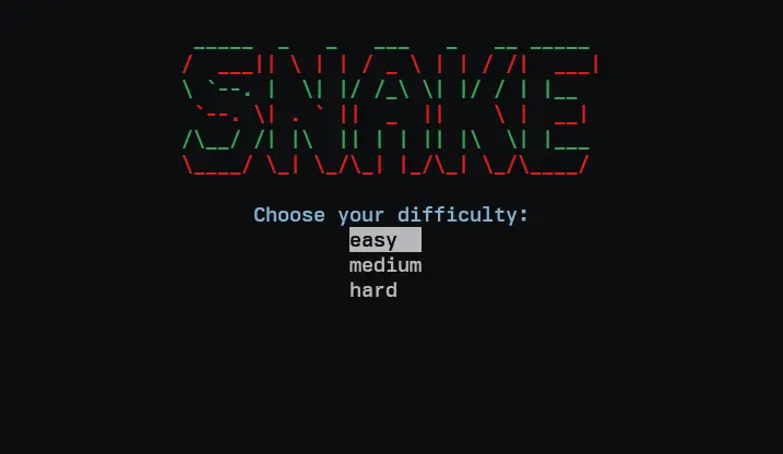
Start Screen

Nothing fancy. The up/down arrow keys navigate the mode menu. ENTER triggers selection.

Game Over Screen

After writing the start screen, the game over screen is a walk in the park. The game over screen only needs to display a banner along with text showing the player’s score. An exit prompt assists with program exit.

void DrawGameOverScreen(const snake::game::SnakeGame& game) {
    clear();

    snake::game::ScreenDimension dim = game.GetScreenDimension();

    /* display the game over banner */
    const std::vector<std::string> kGameOverBanner = {
        " _____   ___  ___  ___ _____ ",
        "|  __ \\ / _ \\ |  \\/  ||  ___|",
        "| |  \\// /_\\ \\| .  . || |__  ",
        "| | __ |  _  || |\\/| ||  __| ",
        "| |_\\ \\| | | || |  | || |___ ",
        " \\____/\\_| |_/\\_|  |_/\\____/ ",
        " _____  _   _  _____ ______  ",
        "|  _  || | | ||  ___|| ___ \\ ",
        "| | | || | | || |__  | |_/ / ",
        "| | | || | | ||  __| |    /  ",
        "\\ \\_/ /\\ \\_/ /| |___ | |\\ \\  ",
        " \\___/  \\___/ \\____/ \\_| \\_| ",
    };
    attron(A_BOLD);
    for (std::size_t i = 0; i < kGameOverBanner.size(); ++i) {
        if (i & 1) {
            attron(COLOR_PAIR(Color::kRed));
        } else {
            attron(COLOR_PAIR(Color::kGreen));
        }

        mvprintw(static_cast<int>(i),
                 (dim.width - static_cast<int>(kGameOverBanner[i].size())) / 2,
                 "%s\n", kGameOverBanner[i].c_str());

        if (i & 1) {
            attroff(COLOR_PAIR(Color::kRed));
        } else {
            attroff(COLOR_PAIR(Color::kGreen));
        }
    }
    attroff(A_BOLD);

    /* display the player's score */
    attron(COLOR_PAIR(Color::kCyan) | A_BOLD);
    const std::string kScoreBanner("SCORE");
    mvprintw(static_cast<int>(kGameOverBanner.size()) + 2,
             (dim.width - static_cast<int>(kScoreBanner.size())) / 2,
             "%s: %d\n", kScoreBanner.c_str(), game.GetScore());
    attroff(COLOR_PAIR(Color::kCyan) | A_BOLD);

    /* display the quit banner */
    const std::string kQuitBanner("press q to quit");
    mvprintw(dim.height - 1, 0, "%s", kQuitBanner.c_str());

    /* wait for the user to enter 'q' before quitting */
    int c = 0;
    while ((c = getch()) != 'q') {
    }
}

And the final result:
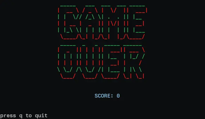
Game Over Screen

The Game Screen

Finally, you get to the most exciting of the three screens: the game screen. In the game screen, you need to draw the snake, target, and the border around the arena. You render the target as a single red diamond. The snake head is an angle bracket whose pointy end tells the player the direction the snake is moving. Character ‘O’ represents the snake’s body.

static void DrawTarget(const snake::game::SnakeGame& game) {
    snake::game::Tile target = game.GetTargetTile();

    attron(COLOR_PAIR(Color::kRed) | A_BOLD);
    mvaddch(target.row, target.col, ACS_DIAMOND);
    attroff(COLOR_PAIR(Color::kRed) | A_BOLD);
}

static void DrawSnake(const snake::game::SnakeGame& game) {
    snake::game::Snake snake = game.GetSnake();

    attron(COLOR_PAIR(Color::kGreen) | A_BOLD);
    const auto& head = snake.front();
    switch (head.direction) {
        case snake::game::Direction::kUp:
            mvaddch(head.row, head.col, '^');
            break;
        case snake::game::Direction::kDown:
            mvaddch(head.row, head.col, 'v');
            break;
        case snake::game::Direction::kLeft:
            mvaddch(head.row, head.col, '<');
            break;
        case snake::game::Direction::kRight:
            mvaddch(head.row, head.col, '>');
            break;
        case snake::game::Direction::kNone:
            mvaddch(head.row, head.col, '?');
            break;
    }

    for (std::size_t i = 1; i < snake.size(); ++i) {
        mvaddch(snake[i].row, snake[i].col, 'O');
    }
    attroff(COLOR_PAIR(Color::kGreen) | A_BOLD);
}

void DrawSnakeScreen(const snake::game::SnakeGame& game) {
    clear();

    if (game.GetBorder()) {
        box(stdscr, 0, 0);
    }
    DrawTarget(game);
    DrawSnake(game);

    refresh();
}

And the rendering:
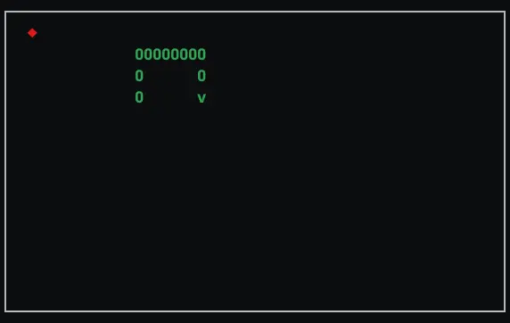
Game Screen

Putting It All Together

The glue that ties all the game logic and graphical elements is in the program main().

int main() {
    /* configure the screen */
    snake::game::ScreenDimension screen_dim = snake::graphics::InitScreen();

    /* display the start menu and fetch the user's game mode selection */
    snake::graphics::GameMode mode = snake::graphics::PromptForGameMode();

    /* draw the initial game screen */
    snake::game::SnakeGame game(screen_dim);
    snake::graphics::DrawSnakeScreen(game);

    RunGameLoop(game, mode);

    /* show the game over screen with the score and exit */
    snake::graphics::DrawGameOverScreen(game);
    snake::graphics::TerminateScreen();

    return 0;
}

The program prompts the user to select their difficulty, runs a game loop which terminates when the player wins or loses, and then renders the game over screen before exiting.

Here’s RunGameLoop()’s implementation:

void RunGameLoop(snake::game::SnakeGame& game,
                 const snake::graphics::GameMode& mode) {
    /* adjust the input delay in order tick the game faster or slower */
    const int kEasyModeDelayMs = 150;
    const int kMedModeDelayMs = 100;
    const int kHardModeDelayMs = 75;
    switch (mode) {
        case snake::graphics::GameMode::kEasy:
            snake::graphics::EnableInputDelay(kEasyModeDelayMs);
            break;
        case snake::graphics::GameMode::kMedium:
            snake::graphics::EnableInputDelay(kMedModeDelayMs);
            break;
        case snake::graphics::GameMode::kHard:
            snake::graphics::EnableInputDelay(kHardModeDelayMs);
            break;
    }

    snake::game::Direction curr_direction = game.GetSnake().front().direction;
    while (!game.GameOver()) {
        snake::game::Direction new_direction = snake::graphics::ReadKeypad();

        /* update the direction only if the user provided one */
        if (new_direction != snake::game::Direction::kNone) {
            curr_direction = new_direction;
        }
        game.Tick(curr_direction);
        snake::graphics::DrawSnakeScreen(game);
    }
    snake::graphics::DisableInputDelay();
}

Adjust difficulty by altering the input delay. The longer the delay, the longer the player has to provide an input before the next game tick executes. If the player fails to provide an input, the snake will continue to move in the direction it’s currently facing.

Conclusion
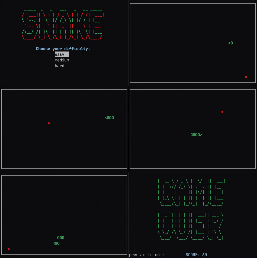
Playing Snake

Ncurses is a solid library. It’s not the most straightforward API out there but there are excellent resources with plenty of examples to get you going. Implementing the snake game logic is a good exercise. That said, the most satisfying part of this project is design of the various views and displays. Watching a crudely animated snake move across the screen never loses its luster.

The complete project source with build instructions, usage, etc. is available on GitHub under snake.

read more →

Resumes in LaTeX

Writing a resume can be a time consuming task involving many rounds of proofreading, recollection, and wordsmithing. Alongside the content, the format of a resume carries a lot of weight. Many people start out writing their resume in Microsoft Word. As their resume evolves, they begin to fiddle with settings buried deep within Words’ menus. It can become tedious.

You may have heard of LaTeX. LaTeX gives you fine-grained control that, at least for a programmer, may be easier to grok than clicking through a series of nested menus. This article takes a look at a LaTeX resume template in the style of Gayle McDowell’s “This Is What a GOOD Resume Should Look Like”. You’ll also see the tools and workflow that simplify resume development in LaTeX.

The Template

To be clear, the template given here isn’t golden but it’s a solid starting point for many. This resume template’s target audience is tech recruiters. That said, most STEM folks can modify this template to suit their particular audience.

Here’s the template in all its glory. Add, remove, and edit as needed in your text editor or LaTeX IDE:

\documentclass[11pt,letterpaper]{article}

\usepackage{enumitem}
\usepackage[dvipsnames]{xcolor}
\usepackage[paper=letterpaper,margin=1in]{geometry}
\usepackage{hyperref}
\usepackage{mathptmx}

\hypersetup{
    pdfcreator={Ivan Guerra},
    pdfproducer={Ivan Guerra},
    pdftitle={Ivan Eduardo Guerra - Resume},
    pdfauthor={Ivan Guerra},
    pdfsubject={Resume},
    colorlinks=true,
    linkcolor=NavyBlue,
    urlcolor=NavyBlue
}

\begin{document}
\newgeometry{top=0.25in, bottom=0.25in, right=0.5in, left=0.5in}

\hrule
\begin{center}
	\begin{LARGE}
		\textbf{Ivan Eduardo Guerra}
	\end{LARGE}
\end{center}
\hrule

\medskip

\begin{minipage}[t]{0.5\textwidth}
	\begin{flushleft}
		\textbf{Contact Information:}\\
		Location: Los Angeles, CA\\
		Mobile Phone \#: (580) 341-8882\\
		E-mail:
		\href{mailto:ivan.eduardo.guerra@gmail.com}{ivan.eduardo.guerra@gmail.com}
	\end{flushleft}
\end{minipage}
\begin{minipage}[t]{0.46\textwidth}
	\begin{flushright}
		\begin{flushleft}
			\textbf{Social Media:}\\
			Personal Site: \url{www.programmador.com}\\
			GitHub: \url{www.github.com/ivan-guerra}\\
			LinkedIn: \url{www.linkedin.com/in/ivan-guerra}
		\end{flushleft}
	\end{flushright}
\end{minipage}

\medskip

\begin{large}
	\textbf{Professional Experience}
\end{large}

\smallskip \hrule \medskip

\begin{minipage}[t]{0.53\textwidth}
	\begin{flushleft}
		\textbf{Northrop Grumman - Aeronautics Systems}\\
		\textbf{\textit{Principal Software Engineer (Active DoD Secret)}}\\
	\end{flushleft}
\end{minipage}
\begin{minipage}[t]{0.43\textwidth}
	\begin{flushright}
		\textbf{September 2019 - Present}
	\end{flushright}
\end{minipage}

\begin{itemize}[noitemsep,topsep=0pt]
	\setlength\itemsep{0.2em}
	\item Led a team of 3 in the development of a Cross Channel Data Link in
	      a real-time Linux environment reducing the probability of unmanned
	      air vehicle loss of control by over 10\%.
	\item Tuned real-time Linux systems on both consumer and proprietary
	      hardware solutions in an effort to reduce worst case latencies.
	      Results drove the selection of safety critical vehicle components.
	\item Deployed and benchmarked autocoded Simulink flight models to
	      various embedded ARM devices including NXP's iMX6 and Xilinx's Zynq
	      UltraScale+ MPSoC.
	\item Employed oscilliscopes, multimeters, and other hardware when
	      debugging and benchmarking avionics software.
	\item Accelerated the development of multiple vehicles by creating
	      reusable Linux and Windows device drivers for a variety of sensors
	      including inertial measurement units, air data computers, and motor
	      controllers.
	\item Designed and implemented a vehicle hardware in the loop testbench
	      reducing flight test risk and providing a means to regression
	      test the system.
	\item Negotiated with suppliers on the software specifications for the next
	      generation of flight control computers used in low cost UAV
	      demonstrators. These UAV demonstrators would drive the capture of
	      future contracts.
\end{itemize}

\medskip

\begin{minipage}[t]{0.53\textwidth}
	\begin{flushleft}
		\textbf{Raytheon - Space and Airborne Systems}\\
		\textbf{\textit{Software Engineer II}}\\
	\end{flushleft}
\end{minipage}
\begin{minipage}[t]{0.43\textwidth}
	\begin{flushright}
		\textbf{June 2017 - September 2019}
	\end{flushright}
\end{minipage}

\begin{itemize}[noitemsep,topsep=0pt]
	\setlength\itemsep{0.2em}
	\item Reduced the time needed to identify software defects during flight
	      tests by implementing an air vehicle software instrumentation API in
	      C++.
	\item Improved laser deconfliction system by implementing SAT location
	      caching. The average time to detect an unwanted laser intersection
	      with a satellite improved by an order of magnitude.
	\item Built a Jenkins CI pipeline to isolate faults and give developers
	      early feedback on code changes.
\end{itemize}

\medskip

\begin{large}
	\textbf{Education}
\end{large}

\smallskip \hrule \medskip

\begin{minipage}[t]{0.5\textwidth}
	\begin{flushleft}
		\textbf{University of Oklahoma: Norman, OK}\\

	\end{flushleft}
\end{minipage}
\begin{minipage}[t]{0.46\textwidth}
	\begin{flushright}
		\textbf{Fall 2013 - Spring 2017}

	\end{flushright}
\end{minipage}
\begin{itemize}[topsep=0pt]
	\setlength\itemsep{0.2em}
	\item B.S.E. in Computer Science with minors in Mathematics and Spanish;
	      Overall GPA: \textbf{3.95}/{4.00}
\end{itemize}

\medskip

\begin{large}
	\textbf{Languages and Technologies}
\end{large}

\smallskip \hrule \medskip

\begin{itemize}[topsep=0pt]
	\setlength\itemsep{0.2em}
	\item \textbf{Languages}: C/C++ (proficient),
	      Python (proficient),
	      Bash (proficient),
	      Rust (competent)
	\item \textbf{Tools and Platforms}: Linux,
	      Realtime Linux,
	      Embedded ARM,
	      FreeRTOS,
	      Docker,
	      GoogleTest,
	      CMake,
	      Git,
	      Subversion,
	      Atlassian Stack
	\item \textbf{Protocols and Standards}: UART,
	      I2C,
	      SPI,
	      CAN,
	      PWM,
	      RS422/485,
	      TCP/UDP,
	      MIL-1553,
	      ARINC 429,
	      WOSA,
	      STANAG 4586,
	      UCI
\end{itemize}

\medskip

\begin{large}
	\textbf{Technical Projects}
\end{large}

\smallskip \hrule \medskip

\begin{itemize}[topsep=0pt]
	\setlength\itemsep{0.2em}
	\item \textbf{\href{https://github.com/ivan-guerra/gsync.git}{gsync}}
	      (2023). GPIO driven synchronization on a real-time Linux system. C/C++,
	      Bash
	\item \textbf{\href{https://github.com/ivan-guerra/steganography.git}{steganography}}
	      (2023). An image based steganography command line tool. C++, Boost
	\item \textbf{\href{https://github.com/ivan-guerra/cpplox.git}{cpplox}}
	      (2022). A C++ implementation of the Lox programming language. C++,
	      Python
	\item \textbf{
		      \href{https://github.com/ivan-guerra/cosmo.git}{cosmo}}
	      (2022). Custom x86 operating system written from scratch. C/C++, x86
	      ASM, Bash
\end{itemize}

\end{document}

Here’s a capture showing how the LaTeX source looks when compiled into a PDF:

Resume as PDF

Building the Resume

You can compile LaTeX source into various document formats. One of the most popular and appropriate for resumes is PDF. A frustrating aspect of working with LaTeX is the sheer number of packages required to get a working distribution capable of taking a vanilla *.tex and transforming it into a PDF.

Docker can prove useful when containerizing a toolchain. Containerizing the over 1GB in dependencies LaTeX requires is a good idea. The following Dockerfile does just that:

FROM ubuntu:latest

ARG DEBIAN_FRONTEND=noninteractive

RUN apt-get update && \
    apt-get install --yes \
        texlive-base \
        texlive-latex-extra

RUN mkdir -p /mnt/resume

WORKDIR /mnt/resume

You can build a LaTeX Docker image with the following command:

docker build . -t latex

Now, when you want to edit your resume, you can launch a container with the directory containing your *.tex file mounted as a volume:

docker run \
    --rm \
    -it \
    --privileged \
    -v $(pwd):/mnt/resume \
    latex:latest

This command will drop you in a Bash shell within the container. The command assumes your *.tex file is in your current working directory. You call the pdflatex program from within the container to transform the *.tex source into a PDF:

pdflatex ivan_guerra_resume.tex

The Workflow

Below is a summary of the resume edit-compile-view cycle:

  1. Place the *.tex file and the Dockerfile in a common directory.
  2. Build the latex Docker image.
  3. Launch a latex container with the directory containing your LaTeX source files mounted as a volume (see the docker run command in the previous section).
  4. Open the *.tex file in a text editor on the host.
  5. Edit the document.
  6. Compile the *.tex file into a PDF from the container shell using pdflatex.
  7. View the output PDF in a PDF viewer or browser on the host. You can leave the document open in your viewer so that when you run pdflatex you see the updates instantly take effect.
  8. Back to (5).

Conclusion

Writing a resume can be hard. You can ease the pain of formatting your resume using powerful tools such as LaTeX. This article provides you with a template resume and workflow for building your next resume in LaTeX. Hope this helps in your next job search!

You can find this template along with many of the scripts and sources referenced in this article on GitHub under resume.

read more →

GPIO Driven Synchronization

Have you ever heard of the Kuramoto Model? The Kuramoto Model Wikipedia page has an impressive video showing out of phase metronomes synchronizing:

Could two or more computers synchronize in a similar fashion? What would be the common “fabric” between the machines? In the clip with the metronomes, the base board is crucial in bringing the metronomes into phase. Perhaps you could use GPIO signals to achieve a similar link between two computers.

Architecting a Test

At a high level, you want to solve the problem of synchronizing two identical, cyclic tasks running on separate but identical hardware. A 1Hz task that blinks an LED would be an appropriate test program. The goal would be to run the blink program on both machines and, through the magic of the Kuramoto Model, the two LEDs would eventually blink in unison.

How would one computer communicate when it last ran to other? You can connect the output GPIO that drives the LED to an input GPIO on the peer board! Below is a sketch of the setup:

graph LR
    %% BeagleBone Black 1 subgraph
    subgraph "BeagleBone Black 1"
        direction TB
        bbb1_gtimer["gtimer"]
        bbb1_gsync["gsync"]
        bbb1_sm["Shared Memory"]

        bbb1_gtimer --> bbb1_sm
        bbb1_sm --> bbb1_gsync
    end

    %% BeagleBone Black 2 subgraph
    subgraph "BeagleBone Black 2"
        direction TB
        bbb2_gtimer["gtimer"]
        bbb2_gsync["gsync"]
        bbb2_sm["Shared Memory"]

        bbb2_gtimer --> bbb2_sm
        bbb2_sm --> bbb2_gsync
    end

    %% External connections between the boards
    bbb1_gsync -->|BBB1_GPIO_OUT| bbb2_gtimer
    bbb2_gsync -->|BBB2_GPIO_OUT| bbb1_gtimer

Each BBB would host two processes: gtimer and gsync. The gtimer process monitors an input GPIO. gtimer blocks on the GPIO waiting for a rising edge event. When the input GPIO goes high, gtimer logs the time when the signal arrived in shared memory. Here’s a flowchart showing how gtimer does its thing:

graph LR
    init_shmem["Init Shmem"] --> init_gpio["Init Input GPIO"]
    init_gpio --> wait_edge["Wait for Rising Edge Event"]
    wait_edge --> write_time["Write Wakeup Time to Shmem"]
    write_time --> wait_edge

gsync is essentially the blink program. gsync runs at a configurable rate, in this case 1Hz. gsync will immediately signal to its peer wakeup has occurred using an output GPIO. gsync then proceeds to read shared memory to know when its peer last ran. Using its own wakeup time and peer wakeup time, gsync can run the Kuramoto Model to compute a wakeup timer delta. The next wakeup time will be closer to bringing the process into sync with its peer. Here’s a flowchart showing how gsync works:

flowchart LR
    attach["Attached to Shmem"] --> init_gpio["Init Output GPIO"]
    init_gpio --> get_time["Get CLOCK_MONOTONIC Time"]
    get_time --> send_signal["Send Wakeup Signal to Peer"]
    send_signal --> compute_time["Compute Next Wakeup Time"]
    compute_time --> sleep["Sleep Until Next Wakeup"]
    sleep --> get_time

The best implementation of gsync and gtimer isn’t immediately obvious. However, the hardware setup is pretty straightforward so lets look at that first.

Hardware Test Setup

You need two computers with which to test. The Beaglebone Black (BBB) single board computer is a good choice. The BBB is a good candidate for the following reasons:

  1. High availability.
  2. The BBB has a ton of unallocated GPIOs.
  3. The BBB runs Linux and so you can use the usual dev tools to build and deploy software.

The circuit below describes the hardware interconnect:

Sync Circuit

P9_15 is the input GPIO and P9_23 is the output GPIO. You can choose other pins if you like. Notice that the input and output GPIOs cross. That is, BBB1’s output GPIO is BBB2’s input GPIO and vice versa. A 470 Ohm resistor limits current to the LED. The resistor also serves as short circuit protection in case the GPIOs mistakenly are both outputs with one side set high and the other set low.

Speaking of GPIO configuration, many of the pins on the BBB support multiple functions. Chapter 6 of the book “Exploring BeagleBone” gives nice coverage of how to configure the GPIOs on the BBB. Verify P9_15 and P9_23 are free. You must configure the pins as GPIO with internal pull down resistors enabled (mux mode 7). If you choose to use different pins, make sure you configure them correctly before powering the circuit!

Doing Things Real-time

To achieve half decent sync results, execute gtimer and gsync as real-time processes on a Linux kernel supporting preemption. The task of configuring and building an RT Linux kernel is nontrivial even in 2023. The bbb_kernel_builder project streamlines the process of building a Linux kernel for the BBB with the PREEMPT_RT patches applied.

There’s more to setting up a real-time Linux application than configuring and building the kernel. A lot more. “Real-Time Linux App Development” goes into the details. The article provides a checklist of all the tweaks you can make at the system and source code level to achieve deterministic behavior. Both the gtimer and gsync implementations follow the guidelines given in the linked article:

  • Prefault heap and stack memory.
  • Lock pages to memory and disable mmap usage.
  • Configure inter-process mutexes with the PTHREAD_PRIO_INHERIT and PTHREAD_PROCESS_SHARED attributes.
  • Set cyclic tasks to use absolute time values as their next wakeup. Reference the CLOCK_MONOTONIC clock for time.

You don’t need to hardcode the scheduling policy and priorities in the source. Instead, you can use the chrt utility to set those parameters up from the run script:

#!/bin/bash

GPIO_DEVNAME="/dev/gpiochip1"
GPIO_IN_OFFSET=16
GPIO_OUT_OFFSET=17
SHMEMKEY=57005
GTIMER_PRIO=80
GSYNC_PRIO=70
FREQ_HZ=1
COUPLING_CONST=0.5

chrt --fifo $GTIMER_PRIO ./gtimer $GPIO_DEVNAME $GPIO_IN_OFFSET $SHMEMKEY &

chrt --fifo $GSYNC_PRIO \
    ./gsync -f $FREQ_HZ -k $COUPLING_CONST $GPIO_DEVNAME $GPIO_OUT_OFFSET \
            $SHMEMKEY &

SCHED_FIFO was the most appropriate RT scheduling policy for this application. gtimer has a higher priority than gsync because you want to log the time when the peer signal arrives ASAP. That means that gtimer may have to preempt a running gsync.

One thing you’d usually do on a multicore system is allocate your cores among the real-time processes. The BBB is a single core system meaning your RT processes get to run on the same core as all the SCHED_OTHER tasks. There’s not much you can do about this. That said, the code is portable to other systems running Linux. An interesting follow-up experiment would be porting this project to a multicore platform. You could dedicate a core to each RT process and compare the measured latencies with those presented at the end of this article.

GPIO Woes

One of the more tedious parts of implementing this sync concept is getting software control of the GPIOs right. You might start with the legacy sysfs API for GPIO control. The general idea is that you can control the behavior and state of a GPIO pin by writing/reading data in a number of different text files. You can export GPIOs to /sys/class/gpio/export. You compute the GPIO number using the formula GPIO_NUM = (32 * CHIPNUM) + OFFSET. After exporting the GPIO, you get a nice file structure like the one shown below:

root@gsync:~# ls /sys/class/gpio/gpio48
active_low device direction edge label power subsystem uevent value

In the snippet, you have the property files for gpio48 AKA GPIO1_16 (chip 1/offset 16) associated with the BBB header pin labeled P9_15. If you wanted to set the pin to be an output pin, you could write out to the direction file:

echo out > /sys/class/gpio/gpio48/direction

If you wanted to set the pin high, you could write 1 to the value file:

echo 1 > /sys/class/gpio/gpio48/value

You get the idea. The sysfs method of GPIO control is nice for one-and-done configurations. That said, you can imagine that opening and closing a file every time you want to toggle a pin is pretty inefficient. You might get away with it running at 1Hz but if you ever decide to up the rate, repeated file IO is going to hurt performance.

So what’s the best way of controlling GPIOs from userspace these days? The answer is libgpiod. libgpiod uses the character device interface to the GPIOs. You don’t lose any of the functionality you had with the sysfs API and you don’t have to deal with the ioctl-based kernel-userpace interaction directly. It even gets bonus points for coming with C++ bindings and a set of useful examples. It’s hard to misuse the API since it throws exceptions for every imaginable error. The time efficiency in toggling a GPIO is also optimal.

The Kuramoto Model

Finally, it’s time to implement the Kuramoto Model. Step one is to translate the equation from the wiki page to something manageable in the code. Here’s the original equation:

dθidt=ωi+KNj=1Nsin(θjθi)\frac{d\theta_i}{dt} = \omega_i + \frac{K}{N}\sum_{j=1}^{N}\sin(\theta_j - \theta_i)

Phase Angles and Time

One thing is immediately apparent: you need a way to convert time to phase angles and vice versa. Your blink task has a known frequency of 1 Hertz meaning one complete task cycle takes 1 second. You can map portions of the cycle in seconds to angles on the unit circle. For example,

  • 0.0000.00 \rightarrow 0 radians
  • 0.25π20.25 \rightarrow \frac{\pi}{2} radians
  • 0.50π0.50 \rightarrow \pi radians
  • 0.753π20.75 \rightarrow \frac{3\pi}{2} radians
  • 1.002π1.00 \rightarrow 2\pi radians

The relationship between time, tt, and frequency, FF, is

t=1Ft = \frac{1}{F}

You’re interested in the time it takes to move through some angle θ\theta in radians. What you find is that

t=θ2πFt = \frac{\theta}{2\pi F}

To go from time to angle, solve for θ\theta:

θ=2πFt\theta = 2\pi Ft

Note that tt is in units of seconds. The gsync implementation tracks time in units of nanoseconds. The conversion equations used in the code account for the units change.

The Wakeup Delta

At this point, you’re ready to plug some numbers into the base equation to compute dθidt\frac{d\theta_i}{dt}. Fill in the terms:

  • ωi\omega_i — This is your base frequency. In radians, the base frequency is 2π2\pi.
  • KK — This is the coupling constant and is a tunable parameter. gsync defaults to K=0.5K = 0.5.
  • NN — This is the number of participants. Since you are syncing two computers, N=2N = 2.
  • θj\theta_j — This is your peer’s phase offset from the ideal base frequency. You can compute θj\theta_j by taking your peer’s reported wakeup time and converting it to a phase angle using the conversion function previously derived.
  • θi\theta_i — This is your own phase offset. Similar to θj\theta_j, θi\theta_i converts your actual wakeup time to a phase angle. To explain a bit further, you have an expected and an actual wakeup time on the computer. The expected time is the time you would execute if there were no additional latencies imposed by the system. The actual wakeup time is the measured time after you resume execution. In short, you’re out of phase with the desired base frequency, and the model uses θi\theta_i to account for that.

In the code, the sync function takes as input the computer’s actual wakeup time and the last reported peer wakeup time extracted from shared memory. Using the latter information, along with frequency and coupling constant info given at program startup, gsync computes dθidt\frac{d\theta_i}{dt} and converts it to a time in nanoseconds. That time is an offset to the next gsync wakeup time.

As an example, suppose gsync ran with a frequency of 1 Hz1\ \text{Hz}, or once every second. Also suppose the sync function returned time deltas in seconds. If the sync function returned a time delta of 0.5-0.5, then gsync would next sleep for

10.5=0.5 seconds1 - 0.5 = 0.5\ \text{seconds}

That is, gsync will wake up earlier by half a second. Maybe the sync function overshot. In the next run, the sync function returns a delta of 0.80.8, so gsync will sleep for

1.0+0.8=1.8 seconds1.0 + 0.8 = 1.8\ \text{seconds}

That is, it will wake up later. Essentially, the delta in the computers’ wakeup times oscillates about 00. The smaller the oscillations, the better the sync.

The End Result

In the end, what do you see? Well, running gtimer and gsync on both BBBs with the frequency of gtimer set to 1 Hz1\ \text{Hz} and the coupling constant set to 0.50.5, you see two LEDs blinking synchronously. It takes maybe 3 to 4 cycles (blinks) before they flash in unison. Running both processes for a day doesn’t produce any noticeable hiccups in the sync!

You can also play a bit with the coupling constant to see what sort of effect it has. You can increment the coupling constant in steps of 0.10.1, starting at K=0.1K = 0.1. What you’ll find is that if KK is too low, the LEDs never seem to synchronize. After crossing a threshold value, synchronization always seems to occur.

So the sync at 1Hz “looks good enough.” Still, it would be interesting to measure using an oscilloscope the delay between the rising edge of one computer’s signal versus the other’s. You can experiment with a number of different rates starting at 1Hz and ramping up to about 500Hz in increments of 50Hz. Below is a histogram of the time deltas you would encounter on a 100Hz run:

100Hz Run

With about 20,000 samples, the average delay was ~100 usec. More interesting than the average is the absolute maximum delay which was approximately 572 usec. These observations more or less held true for all test runs in the range [1, 400] Hertz.

Beyond the 400Hz run rate, you start to see some oddball results. Below is a capture of a 500Hz run:

500Hz Run

The average delta was still approximately 100 usec. The maximum delta saw huge spikes around 2.7 ms. Worse yet, these were more than just a few outliers, there were multiple hits in the 2.5 ms range. Are the spikes driven by weak coupling? Is there a timing bug between gtimer and gsync? Questions for another day.

Conclusion

Synchronizing at least two computers linked via only GPIO is possible. Better yet, the Kuramoto Model used to bring the two machines into phase is relatively straightforward to code and reason about. Moreover, submillisecond synchronization is achievable for rates below 500Hz on bargain hardware using free and open source software.

The complete project source with build instructions, usage, etc. is available on GitHub under gsync.

read more →

Beaglebone Black WiFi Setup

When developing on the Beaglebone Black (BBB), it’s handy to have the board on the network for when you want to SSH into it, install packages, etc. That said, you may not want to run an Ethernet cable from the BBB to a switch. Luckily, the BBB has support for a number of WiFi adapters. I purchased the EDIMAX EQ-7811UN adapter and set about trying to connect a BBB to my local network. This article walks through the steps required to get connected. These instructions also apply to the BBB wireless variants (that is, those BBBs with a wireless chip).

Beaglebone Black WiFi Configuration

The steps below assume use of a supported WiFi dongle on an official BBB image and require root access.

  1. Boot the BBB with the WiFi adapter plugged into the USB port. The official BBB site recommends running off DC power when utilizing the adapter due the adapter’s current requirements.

  2. Run the command line network manager:

sudo connmanctl

You can ignore the Error getting VPN connections: The name net.connman.vpn was not provided by any .service files message.

  1. Enable WiFi:
connmanctl> enable wifi
  1. Scan for WiFi networks:
connmanctl> scan wifi
  1. Show available WiFi services:
connmanctl> services

If you don’t see any services, you can disable WiFi tethering and try again:

connmanctl> tether wifi off
connmanctl> services
  1. Turn on the agent:
connmanctl> agent on
  1. Connect to your WiFi/service. Replace WIFI_HASH with the string from step 5 that corresponds to your WiFi network:
connmanctl> connect WIFI_HASH
  1. Enter your WiFi password:
Passphrase?
  1. Verify you have autoconnect enabled:
connmanctl> services

You should see *AO or *AR next to your network’s name.

  1. Exit connmanctl:
connmanctl> quit
  1. Verify you’re connected. Try pinging gnu.org:
ping gnu.org
  1. By default, connman will use DHCP to retrieve an IP. If instead you’d like to set a static IP, run the command below replacing the WIFI_HASH, IP_ADDR, SUBNET_MASK, and GATEWAY_ADDR with values corresponding to your network:
connmanctl> config WIFI_HASH --ipv4 manual IP_ADDR SUBNET_MASK GATEWAY_ADDR
read more →

Linux USB Serial Device Name Binding

Have you worked with USB serial devices on Linux? One annoyance you may have come across is device name changes after each reboot. This problem gets solved by binding a custom /dev name to a USB device. This post shows you how.

To be clear, this article walks through assigning USB serial devices persistent names. If you have a USB block device and would like to give it a persistent name, the ArchWiki has you covered.

USB Serial Device Name Binding Using udev

The instructions below will work on a Linux distro that uses udev for device management. You will need root privileges to follow these instructions!

  1. Plugin the USB serial device.
  2. Identify the /dev/ttyUSB* name assigned to your device. There are many ways to do this. Perhaps the easiest is to grep the dmesg log to see what name the kernel gives the device:
dmesg | grep USB
  1. List the device attributes using udevadm. Replace <X> with the USB number found in step 2:
udevadm info --name=/dev/ttyUSB<X> --attribute-walk
  1. You’ll see a list of attributes for your device on the console. Find one or more attributes that uniquely identify your device. The combination of vendor ID and product ID is a good choice.
  2. Create or edit the /etc/udev/rules.d/99-usb-serial.rules file to include an entry like the one shown below. Be sure to input your own attributes and set SYMLINK to the name you’d like the device to have.
SUBSYSTEM=="tty", ATTRS{idVendor}=="067b", ATTRS{idProduct}=="2303", SYMLINK+="mydevice"
  1. Load the new rules using udevadm:
udevadm trigger
  1. Verify the USB serial device has its new name:
ls -l /dev/mydevice
  1. On reboot or when you plugin the device, the new name will persist.

To bind more device names, simply add rules to 99-usb-serial.rules. To undo these changes, delete the device’s corresponding rule in /etc/udev/rules.d/99-usb-serial.rules and run udevadm trigger.

read more →