Are you a fan of the MMO RuneScape? Are you not a fan of the grinds RuneScape subjects its players to? If you answered yes to these two questions, it’s likely botting has crossed your mind.

Put aside that botting is breaks the game’s rules. Creating a scriptable bot that can avoid RuneScape’s bot detection system presents a number of interesting technical problems. This article explores the creation of a rudimentary bot: an auto clicker bot.

Bot Taxonomy

People have been botting RuneScape for ages. In that time, there’s been a number of different flavors of bots. If you search the RS botting forums, you’ll come across references to color bots, injection bots, reflection bots, and more.

Below is a summary of the top three bot types taken directly from the OSRS Botting wiki.

• Color Bots: Color bots are a primitive form of botting that uses colors in the game to perform tasks. The bot is told to recognise a certain type of color on the screen and then the bot clicks on that color.
• Injection Bots: An injection bot is a type of bot that utilises the RuneScape code itself. It injects itself into the RuneScape client and is able to read the client’s code. It makes sense of the code and is able to make choices based on what the code states it will do.
• Reflection Bots: Reflection bots create a mirror image of the RuneScape applet by accessing the loaded classes and then reads the code of the “reflected” copy, without injecting any code.

Color, injection, and reflection bots are often overkill for automating basic tasks. A surprising amount of RS gameplay amounts to clicking the same group of pixels for hours on end. The obvious solution is to implement a scriptable auto clicker. That said, a naive auto clicker will get you banned in the span of a few hours. In the next section, you’ll see what behaviors are speculated to trigger the bot detection system.

Botting Red Flags

What actions lead to a ban? The short answer is, only Jagex’s bot busting team knows. Further, RuneScape 3 and Old School RuneScape have separate bot busting teams. It’s likely that their detection mechanisms have overlap but aren’t identical. What follows in this section are best guesses at what the bot detection system considers red flags.

You can think of the bot detection system as a scale. On one side you have a human player and on the other a bot. Tip the scale to the bot side beyond a certain threshold and an automatic ban gets applied to your account. Listed below are a few of the behaviors that are thought to tip the scales towards bot:

• Account Age: More scrutiny gets placed on new accounts as a measure to counter bot farms. Older accounts with hours of manual playtime face less pressure from the bot detection system.
• Inhuman Playtime: Few players can train a single skill for 24 hours straight. Inhuman play streaks are a good botting indicator.
• IP Info: Some speculate that Jagex analyzes IP information. If you play through a VPN used by botters, your IP may raise a red flag.
• Perfect Clicks: If you click the exact same pixel for hours on end, that’s a good sign you’re a bot.
• Robotic Mouse Movement: Jagex can certainly track mouse gestures. Whether they analyze the movements is unknown. A survivable bot must generate human like mouse movements.
• In Game Reports: Other players reporting your account for botting is undesirable.

These are just a few actions that could trigger the bot detection system. If you employ one of the botting strategies that hooks into the game client, there are even more dangers to avoid.

Development Language

The goal is to write an auto clicker bot. Auto clickers don’t hook into the game client and therefore aren’t limited to Java or C++ for development. You should write your auto clicker bot in Python. Python is itself a scripting language that supports a number of popular libraries. Those libraries include APIs for identifying screen dimensions, manipulating the mouse, and random number generation. You’ll need these functions and more to build a survivable bot. Python is also a portable language. Write the script once and it’ll run on Linux, Windows, and MacOS. The auto clicker script linked at the end of this article is 366 lines of Python code with comments included.

Auto Clicker Bot Design

The concept behind an auto clicker bot is simple. You define a set of click events where each click event specifies the mouse button to press and a target screen location. The bot continuously loops over the events until it’s terminated. Implementing such a program in Python takes minutes. It would also only take the RuneScape bot detection system a few hours to ban such a bot. Lets look at how to make this auto clicker bot more survivable.

Randomized Delays

When you train a skill in RuneScape, you click a sequence of UI elements over and over. Do you click those elements at the exact same cadence each time? Of course not. The delay between clicks varies even if only by a few hundreds of milliseconds. To decrease the chance of getting banned, you append a min and max delay in seconds to each click event. After the bot performs a click, it will wait $N$ seconds where $N$ gets chosen at random from the configured delay range.

How big should the range be? Depends on the event and how risk tolerant you are. Rule of thumb is make the bottom end of the range large enough to execute the action to completion then add 5 seconds to that to get the max delay. For example, if it takes 28 seconds to fletch an inventory of logs, you would specify a delay range of $[28, 33]$.

Random Idling

Random idles or breaks can help approximate human like RuneScape gameplay. For example, maybe every 30 minutes you take a 5 minute break to get a snack or load another Youtube video. The auto clicker bot should do the same. Every $N$ minutes, an idle of $M$ seconds gets inserted. Similar to the click event delays, you can specify a range from which to select $M$.

Click Boxes

By now you know that clicking the exact same pixel is a bad idea. An easy way around this is to not hardcode a pixel location but instead define a click box. When the click event executes, a random pixel in the bounds of the box gets selected. A click box doesn’t necessarily need to be a set of four vertices that form a perfect square. It can be any set of four unique vertices. Below is a Python class, ClickBox, that takes four vertices and exposes an API for generating a random point within the quadrilateral formed by those points.

class ClickBox:
    """Define a quadrilateral representing an in game click box.

    To avoid bot detection, don't click the exact same pixel location for hours on end.
    ClickBox provides an API for consistently clicking a target object (e.g., bank chest, NPC, etc.)
    without hardcoding a specific pixel location.
    """

    def __init__(self, vertices: list[tuple[int]]) -> None:
        """Construct a quadrilateral.

        Args:
            vertices: A list of four 2D points representing the corners of the click box.
        Throws:
            ValueError: When the length of the parameter vertices list is not exactly four.
        """
        num_vertices = 4
        if len(vertices) != num_vertices:
            raise ValueError(
                f"invalid number of vertices, expected {num_vertices} got {len(vertices)}")
        self._vertices = vertices

    def _random_point_in_triangle(self, v1, v2, v3) -> tuple[int]:
        """Return a point within the bounds of the triangle formed by the paramater vertices."""
        s = random.random()
        t = random.random()

        # Ensure the point is inside the triangle.
        if s + t > 1:
            s = 1 - s
            t = 1 - t

        x = v1[0] + s * (v2[0] - v1[0]) + t * (v3[0] - v1[0])
        y = v1[1] + s * (v2[1] - v1[1]) + t * (v3[1] - v1[1])

        return (x, y)

    def get_rand_point(self) -> tuple[int]:
        """Return a random point within click box bounds."""
        if random.random() < 0.5:
            # Generate a point in the first triangle.
            return self._random_point_in_triangle(
                self._vertices[0], self._vertices[1], self._vertices[2])
        # Generate a point in the second triangle.
        return self._random_point_in_triangle(
            self._vertices[0], self._vertices[2], self._vertices[3])

The get_rand_point() method selects a random point from one of two triangles formed using the input vertices. The animation below illustrates the concept using a set of vertices that happen to form a perfect square:

Moving the Mouse

You want your mouse movements to be as human like as possible. There are a couple of different Python projects that solve this problem:

• WindMouse: Models mouse movement using an imaginary wind and gravitational force. The implementation is tunable allowing you to adjust the mouse speed and overshoot.
• bezmouse: Models mouse movement using Bezier curves. The mouse moves from point A to B along a random Bezier curve.
• pyHM: Though the implementation isn’t well documented, a quick look at the source shows this is yet another implementation that uses Bezier curves to model mouse movement.

pyHM stands out as the best choice since it’s easiest to use and tune. pyHM’s mouse motions look convincing as well. Below is an animation showing a couple of pyHM mouse gestures with their trace:

Its worth mentioning you can adjust the speed at which the mouse moves from A to B using a multiplier. You should randomize the speed of the mouse movements via an interval.

Conclusion

The rsbot project puts the ideas from the previous sections into practice. The README includes instructions on how to configure and run the bot. The bot has successfully allowed a main account to level fletching, firemaking, and crafting to 99 all in the last month.

The bot has a few shortcomings. In particular, if you change the game camera orientation or screen resolution, you have to regenerate all those click boxes. The project includes a helper script to reduce the tedium around creating an rsbot click event script.

Use the rsbot auto clicker at your own risk. Don’t run the script on an account you wouldn’t be okay losing. Don’t run the bot for inhuman amounts of time. Don’t test your scripts or run the bot in highly populated areas where you can get reported. Do tune the delays and random intervals before setting the bot to run without supervision. Follow these basic rules and you too can save hours in maxing the most tedious skills in RuneScape.

The article “Making Cellular Textures” gives a good description of how you would go about generating textured images like the ones shown below.

The authors’ descriptions and pseudocode provide the basis for the implementation of a CLI texture generator. This article describes such a tool and its performance when generating a number of different textures.

Texture Parameters

The goal of the tool is to generate a texture as an $M \times N$ grayscale PNG. The program exposes five key parameters that control the look of the output image:

Option	Description
--num-points	Controls the number of randomly generated points. AKA the texture points.
--num-neighbors	The number of nearest neighbors whose distance is factored into each pixel’s color calculation.
--dist-op	The operation to apply to the nearest neighbor distances.
--enable-tiling	When computing the distance from pixel to texture point, enable wrapping around the border of the image.
--invert-colors	Invert the color of each pixel before outputting.

The Algorithm

The process for generating a texture is as follows:

• Create a MxN grid of pixels.
• Generate --num-points random texture points. All points must lie within the bounds of the pixel grid.
• For each pixel:
  • Find the --num-neighbors nearest texture points.
  • Calculate the distance from the pixel to each neighboring texture point. If tiling is active, apply a modified distance formula that accounts for wrapping around the edges of the pixel grid.
  • Apply the --dist-op operation to the collection of distances. For example, if in the previous step you computed the distances 1, 2, 3, and your if in the previous step you computed the distances 1, 2, 3, and your --dist-op was multiplication, you would compute dist=1*2*3=6.
  • Cache each pixel’s $dist$ value.
  • Keep track of the minimum and maximum $dist$ values: $mindist$ and
  • Compute the grayscale value of the $i$th pixel, $c_i$:

$$c_i = \frac{dist_i - minDist}{maxDist - minDist} \times 255$$

• Write the pixels to a grayscale PNG output file.

The Layman’s Explanation

The formulas and numbers can get confusing. The core idea is that you are iterating a grid of grayscale pixels. You want to determine how light or dark each pixel should be. You generate a set of random “texture points” within the bounds of the image. Then you find the $k$ nearest texture points of each pixel and apply an arbitrary formula to the collection of distances from each of the $k$ neighbors to the pixel. Applying the formula generates a single “distance” value. You later use this distance value along with the global max and min distances to determine the color of the pixel.

The number of neighbors and the operation you apply creates drastic changes in the output. For example, set --num-neighbors to 2 and --dist-op to minus and you get the following scaly image:

Set --num-neighbors to 1 and --dist-op to multiply and you get the following dotted texture:

The CLI tool is interesting because you can write a script to tweak the parameters generating numerous textures. The video that follows shows some interesting textures generated by running a simple bash script:

#!/bin/bash

for i in $(seq 0 9);
do
    ./ctext 512 512 "sub_1000_$i.png" -k "$i" -d "-"
done

Finding Nearest Neighbors

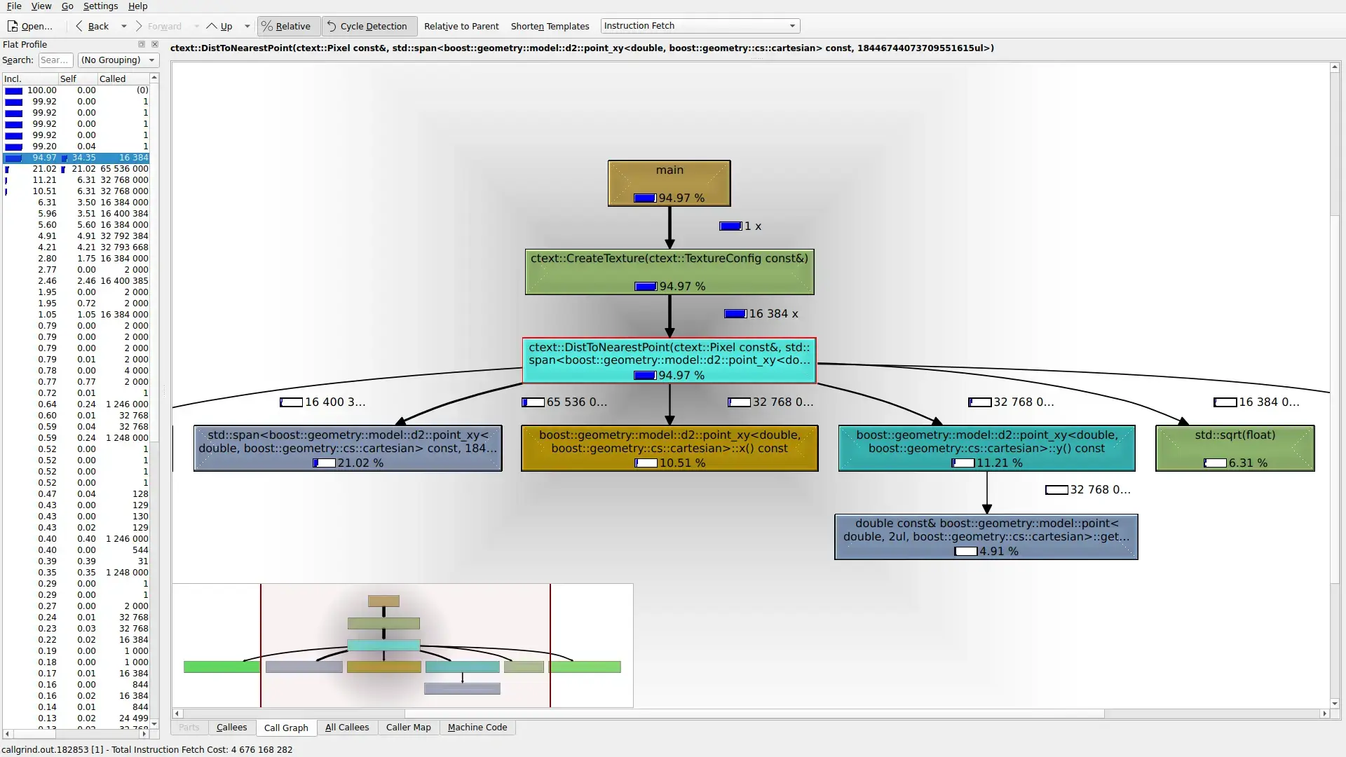
Given a big enough image and enough texture points, texture generation can be a slow process. You spend the majority of the time computing the distance to the nearest neighbors of each pixel as shown in the KCachegrind capture below:

The capture shows a single ctext run:

ctext 128 128 test.png --num-neighbors 1 --dist-op "-"

The run uses a brute force, $\mathcal{O}(n^2)$ algorithm, where $n$ is the number of texture points. number of texture points.

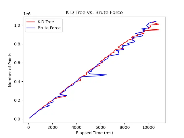
The “Making Cellular Textures” article suggests a number of tree data structures that could help speed up the search. Among these is the K-D Tree. There are a few C++ K-D Tree implementations floating around online. This C++ implementation for nearest neighbor and k nearest neighbors is one of the better options given it comes with solid unit/benchmark tests. You’d think an $\mathcal{O}(\log n)$ nearest neighbor search complexity would grant You’d think a $\mathcal{O}(logn)$ nearest neighbor search complexity would grant a massive speedup. Measurements showed otherwise:

The graph shows the performance of the brute force algorithm versus a 2-D tree on the command

ctext 1024 1024 --num-neighbors=1 --dist-op="-" --num-points=<VARIABLE>

The tree performs about the same or worse in some instances. Why? It’s likely because there’s a significant cost to constructing the tree. The worst case complexity for constructing the tree is $\mathcal{O}(nlog^2n)$. Then add in that the search complexity is on average $\mathcal{O}(logn)$. The distribution of the random points also plays a key role. The more uniformly distributed the points are, the more balanced the tree will be. Some of those large spikes to the right might be the result of searches on a “skewed” tree.

Conclusion

With some basic math and computer science, you can write a CLI tool to help you explore the “cellular texture space.” The end result: some neat looking pictures.

The complete project source is available on GitHub under cellular_textures. Note, this project has since been rewritten in Rust. The Rust version of the program uses a K-D tree for nearest neighbor searches exclusively. The performance of the Rust implementation is comparable to that of the original C++ implementation.

This post includes the notes made while reading the book titled “The Practice of Programming” by Brian Kernighan and Rob Pike.

Chapter 1: Style

• Use descriptive names for globals and short names for locals.
• Consistency with local coding conventions is key.
• Use active names for functions.
• Name boolean functions such that the return value is obvious.
• Indent to show structure. Be consistent with whatever style you choose.
• Use parentheses to resolve ambiguity. Don’t expect the reader to be an expert in precedence rules.
• Break up complex expressions. Don’t cram a bunch into one line just because you can.
• Clarity isn’t the same as brevity. Ease of understanding is what distinguishes the two.
• In C/C++, avoid function macros. Just use a function. Inline or use constexpr as appropriate.
• Give names to magic numbers.
• Don’t use macros for numeric constants. Use enum, const, and constexpr.
• Never hardcode sizes. Use features of the language such as sizeof or size members of a container.
• Comments should avoid stating the obvious, contradicting the code, and should only exist to enhance clarity.

Chapter 2: Algorithms and Data Structures

• Most programs require some form of searching or sorting.

• Linear and binary search are common algorithms that handle searching for an element in a collection. If your language has built-ins for linear/binary search, use them.

• Similar to searching, use your language’s sorting routines rather than rolling out your own. Read the docs to understand not only the API but any gotchas regarding runtime/space complexity.

• Big-oh notation is a tool for describing the time/space complexity of an algorithm. Below is a table of the most common complexities:

  Notation	Name
  $O(1)$	constant
  $O(logn)$	logarithmic
  $O(n)$	linear
  $O(nlogn)$	nlogn
  $O(n^2)$	quadratic
  $O(n^3)$	cubic
  $O(2^n)$	exponential

• Arrays are easy to use, provide $O(1)$ access to any item, work well with binary search and quicksort, and have little space overhead. For fixed sized data sets, or for guaranteed small collections of data, arrays are unbeatable.

• Lists are useful when the container size isn’t known at compile time and when insertions/deletions in the middle of the collection happen frequently. You can’t index a list so operations like searching are always linear.

• Trees represent a hierarchical relationship between a collection of items. The structure of the tree often affects algorithm performance as is the case with a balanced versus unbalanced BST. You can traverse a tree in preorder, inorder, and postorder fashion. Each traversal introduces benefits depending on the contents of the tree.

• Hash tables provide fast (on average $O(1)$) insertion, deletion, and lookup. The performance of a hash table relies on the implementation of its hashing function and collision handling scheme.

Chapter 3: Design and Implementation

• Try to handle irregularities, exceptions and special cases in data. Code is harder to get right so the control flow should be as simple and regular as possible.
• It’s important to choose simple algorithms and data structures, the simplest that will do the job in reasonable time for the expected problem size.
• Start your detailed design thinking about the data structures guided by what algorithms you might use.
• Expect to iterate. Start with something simple and refine it.

Chapter 4: Interfaces

• Creating a prototype that solves a problem is a good first step in understanding how to develop a more thorough design.

• Key concerns when designing are interfaces, information hiding, resource management, and error handling.

• Good interfaces follow a set of principles:

  • Hide implementation details.
  • Choose a small orthogonal set of primitives. Make your interfaces narrow. That is, provide only what’s necessary. Don’t expose multiple ways of doing the same thing.
  • Don’t reach behind the user’s back. Don’t write secret files, variables, or change global data. Try not to modify the caller’s input when possible. Make the interface as self-contained as possible. Don’t inject dependencies where the user must call function A before function B etc.
  • Do the same thing the same way everywhere. Consistency and regularity are important.

• You should always consider how an interface manages resources. Construction, destruction, and copying are of key concern. Try to always free a resource at the same layer that allocated it.

• Try to write reentrant code meaning code that works regardless of the number of simultaneous executions. Avoid global variables, static local variables, and modifying anything that has potential for concurrent access.

• Detect errors at a low level, handle them at a high level. This is especially true for library code.

• Use exceptions for exceptional situations. Avoid using exceptions for control flow.

Chapter 5: Debugging

• The authors don’t recommend use of a debugger. This is counter personal experience in which interactive debugging has been invaluable. Stack traces, breakpoints, etc. make locating and understanding bugs easier. The trouble is in overcoming the learning curve of working with the debugger. It’s worth learning if you program professionally.

• Tips for when you have plenty of “clues” to work with:

  • Look for familiar patterns. Does the bug look like something you’ve seen before?
  • Examine the most recent change. If you edit and test in small increments, a bug will likely be a direct result of the most recent change. Using a version control system makes this easier.
  • Don’t make the same mistake twice. After you fix a bug, ask whether you might have made the same mistake somewhere else.
  • Debug it now not later. It’s easy to forget a bug exists especially if it only appears under specific circumstances.
  • Get a stack trace.
  • Read before typing. Read the code and think about what it’s doing and how your change would play out before making it.
  • Explain your code to someone else. If there’s no one to talk to, just talking about the bug aloud might be good enough.

• Tips when there’s not much information to go off of:

  • Make the bug reproducible.
  • Divide and conquer. Narrow down program inputs and code to the smallest you can while still reliably triggering the bug.
  • Study the numerology of failures. This basically means looking for a pattern in the erroneous output. The patterns can give hints that point you to the source of the issue.
  • Display output to localize your search. This means using print statements to narrow done the source of the error. You should only do this when a debugger isn’t available or the problem would be hard to spot in a debugger (for example a bug to do with multithreaded execution).
  • Write a log file.
  • Draw a picture. Aside from just drawing the data structures or flow of the program, you can also add statistics to the code then generate plots from those statistics for further analysis.
  • Keep records. Write down what you’ve tried so you don’t skip an idea or duplicate effort.

• With non reproducible bugs, you have to consider factors such as variable inputs, environment variables, startup files, random seeds, etc. You have to narrow down what can change between runs.

Chapter 6: Testing

• Testing isn’t the same as debugging.

• Testing can demonstrate the presence of bugs but not their absence.

• Test as you write the code:

  • Test code at its boundaries.
  • Test pre- and post conditions.
  • Use assertions.
  • Program defensively.
  • Check error returns.

• Systematic testing:

  • Test incrementally.
  • Test the simple parts first.
  • Know what output to expect.
  • Verify conservation properties. Some programs should leave properties of the input unchanged. You can use tools like wc, diff, md5sum, etc. to verify those properties.
  • Compare independent implementations.
  • Measure test coverage.

• Automate your testing. Testing frameworks such as GoogleTest and doctest are excellent for writing large test suites.

• Stress tests can introduced inputs that humans would avoid or would be unlikely to provide. The authors’ characterization of stress testing is different than the usual definition where one sends large amounts of valid input to a program hoping to induce a crash.

• Testing tips:

  • Vary your test cases.
  • Don’t keep on implementing new features or even testing existing ones if you know there are bugs.
  • Test output should include all input parameter settings, so the tests can be reproduced exactly.
  • Test on multiple machines, compilers, and operating systems.

Chapter 7: Performance

• The first step in optimizing for performance is determining if there’s a need to optimize at all.

• Use tools to identify bottlenecks. These tools should include timers and profilers.

• Focus your energy on the hotpots. The outputs of the profiler will guide you to the hotspot. Post optimization, measure again and repeat the process for any new hotpots observed.

• Plot benchmark data. Visualizing the data can call to your attention issues that otherwise wouldn’t be apparent from just looking at the numbers.

• Strategies for speed:

  • Use a better algorithm or data structure.
  • Enable compiler optimizations.
  • Tune the code. See next section for tuning tips.
  • Don’t optimize what doesn’t matter.

• Tuning the code:

  • Collect common subexpressions.
  • Replace expensive operations by cheap ones.
  • Unroll or remove loops.
  • Cache frequently used values.
  • Write a special-purpose allocator. Authors refer to essentially object caches/slab allocation.
  • Buffer input and output.
  • Handle special cases separately.
  • Precompute results.
  • Use approximate values.
  • Rewrite in a lower level language.

• Space efficiency:

  • Save space by using the smallest possible data type.
  • Don’t store what you can easily recompute.

Chapter 8: Portability

• A program can be portable between compilers, operating systems, and processor.

• The techniques of portable programming relate to the techniques of good programming in general.

• Languages:

  • An easy way to achieve portability is to stick with the language’s standard.
  • Program in the mainstream. This means give preference to the mature/stable parts of the language.
  • Beware of language trouble spots. These are parts of the language that are intentionally left ambiguous to give the language implementer more leeway in their design.
  • Make no assumptions about type sizes. Use the tools of the language to determine sizes (for example, sizeof).
  • Don’t depend on order of evaluation.
  • Understand what type of shifting the >> and << operators do. Logical versus arithmetic shifting. See this link for the details in C/C++.
  • Don’t write endianness specific code.
  • Don’t make assumptions about the alignment of structures and class members.

• Avoid conditional compilation where possible. Stick to the portable features of the language.

• When you do have nonportable sections of code, separate them into different files under a common interface.

• When it comes to endianness, the endianness of the sending and receiving machines doesn’t matter. What matters is the agreed upon endianness of the data transmission.

• The authors recommend sending data as text. The argument being text is more portable than binary formats. Binary formats do have their place when it comes to saving space and processing efficiency.

• Consider whether a change that breaks portability is worth making. Try to remain backwards compatible whenever possible.

ffmpeg is a powerful command line tool for processing video and audio files. ffmpeg can do just about anything you can imagine with media files. The trouble is in understanding how to invoke the program correctly. There are a few options that require some Linux and multimedia expertise to get right. This article covers a couple handy ffmpeg hacks that have made much of the audio/visual content on this website possible. The commands presented here are MP4 centric. That said, you can modify most of the commands to work with alternative formats (for example, WebM).

Screen Recording

You can use ffmpeg to create a desktop recording. The command below assumes you’re on a Linux machine with an X Server running.

ffmpeg -y -f x11grab -draw_mouse 0 -s $RESOLUTION -i $DISPLAY ${OUTPUT_FILE}.mp4

Lets dissect the options:

Option	Description
-y	Overwrite an existing output file without prompting the User for confirmation.
-f x11grab	Use the x11grab device. This device allows one to capture a region of an X11 display.
-draw_mouse 0	Disables recording of the mouse. Set this to 1 or remove the option completely to include the mouse in the recording.
-s $RESOLUTION	Sets the capture resolution. For example, -s 1920x1080.
-i $DISPLAY	Sets the input X11 display. You likely want to put the value of $DISPLAY here to capture the default X display.
${OUTPUT_FILE}.mp4	The path to the output MP4 file.

If you want to make a recording that includes audio, the command looks a little different:

ffmpeg -y -f x11grab -draw_mouse 0 -s $RESOLUTION -i $DISPLAY -f pulse -ac 2 -i default ${OUTPUT_FILE}.mp4

What does the newly added -f pulse -ac 2 -i default bit do? It tells ffmpeg to record audio using the default PulseAudio device. If you instead use Alsa for audio, replace the PulseAudio device with the equivalent Alsa device: -f alsa -ac 2 -i hw:0. Having trouble identifying your Alsa/PulseAudio device? See “Capture/ALSA” and “Capture/PulseAudio” for help.

You can augment the capture command to change the framerate, recording area, and more. Checkout the original source of this info for more details on how to capture video/audio.

Concatenating Video Files

Suppose you wanted to concatenate a number of recordings. You can use ffmpeg’s concat demuxer to join all the files.

The first step is to create a text file with the list of recordings you want to concat in the order you want them concatenated in:

file record1.mp4
file record2.mp4
file record3.mp4
...

Suppose you had all your *.mp4 files in a directory. You can create ffmpeg’s concat input file using printf:

printf "file $s\n" *.mp4 > mylist.txt

Run ffmpeg using the concat device with your file list as input:

ffmpeg -f concat -i mylist.txt -c copy output.mp4

Note, this command works for files with the same codec. If you want to join files with different codecs, checkout “Concatenation of files with different codecs”.

Adding Text Overlays to Videos

Need to add a small text box to your video? Look no further than the fun command below:

ffmpeg -y -i ${IN}.mp4 -vf "drawtext=:text='Hello World':fontfile=/path/to/font.ttf:fontcolor=white:fontsize=50:box=1:boxcolor=black@0.5:boxborderw=5:x=(w-text_w)/2:y=(h-text_h)/2:enable='between(t,5,10)'" -codec:a copy ${OUT}.mp4

The magic happens in the video filter flag’s "drawtext=..." argument. The fields of the argument are mostly self explanatory though the enable and x/y options could do with a little elaboration.

The enable option specifies a window of time (in seconds) when the text label will be visible. In this example, enable='between(t,5,10)' means the text box will be visible from the 5 second mark to the 10 second mark in the video.

The x/y options specify the location of the text box on screen. The w, h, text_w, and text_h are variables provided by ffmpeg to make it easier to compute a position. w/h are the screen width and height. text_w/text_h are the text string’s width and height.

The drawtext filter takes many more options. Take a look at the official docs for all the details.

Bonus: Video Playback

It’s likely that you want to playback your video after an edit. ffplay is a program that uses ffmpeg libraries and SDL to playback a media file. The following command will play an MP4 adding a small text box with a live timestamp at the bottom:

ffplay -vf "drawtext=text='%{pts\:hms}':box=1:x=(w-tw)/2:y=h-(2*lh)" ${MY_VIDEO}.mp4

This command isn’t limited to MP4s. You can pass any video format ffmpeg supports to ffplay.

Conclusion

This article doesn’t scratch the surface of what’s possible with ffmpeg. That said, these “simple” commands have helped make most of the video content on this site! Hopefully, these same commands save you some time in creating your own video content.

The Ulam spiral is a graphical depiction of a set of prime numbers devised by the mathematician Stanislaw Ulam. To quote the Wiki, it’s constructed by writing the positive integers in a square spiral and specially marking the prime numbers. The outcome is a square with distinct diagonal, horizontal, and vertical lines. This post will walk through the development of a Ulam spiral visualization tool.

Creating a Ulam Spiral

Take a look at the 4x4 Ulam spiral below:

 0  0  0  7
11  2  0  0
 0  3  0  5
13  0  0  0

In this spiral, the composite numbers are output as zero and the prime numbers are output as themselves. The spiral grows counter clockwise from the center.

How do you programmatically generate this spiral? GeeksForGeeks suggests two methods: generation via simulation and generation via dividing the matrix into cycles.

Below is a C++ implementation of the simulation approach:

using RowVect = std::vector<int>;
using SquareLattice = std::vector<RowVect>;

std::optional<SquareLattice> GenerateUlamSpiral(int dim) {
  /* The implementation that follows is a slightly tweaked version of the
   * algorithm given here:
   * https://www.geeksforgeeks.org/print-a-given-matrix-in-spiral-form/# */

  if (dim <= 0) { /* invalid dimension */
    return std::nullopt;
  }

  const std::vector<Position> kDirections = {
      {.row = 0, .col = -1}, /* west */
      {.row = -1, .col = 0}, /* north */
      {.row = 0, .col = 1},  /* east  */
      {.row = 1, .col = 0},  /* south */
  };

  std::unordered_set<int> primes = SieveOfEratosthenes(dim * dim);
  SquareLattice spiral(dim, RowVect(dim, 0));
  Position pos = {.row = dim - 1, .col = dim - 1};
  int dir_index = 0;
  int value = dim * dim;
  std::unordered_set<Position, PositionHash> visited;
  for (int i = 0; i < dim * dim; ++i) {
    /* We always write a number. If value is prime, we write value, otherwise,
     * we write 0 as a placeholder. */
    if (primes.contains(value)) {
      spiral[pos.row][pos.col] = value;
    } else {
      spiral[pos.row][pos.col] = 0;
    }
    value--;

    visited.insert(pos);

    Position candidate = kDirections[dir_index] + pos;
    if (IsInBounds(candidate, dim) && !visited.count(candidate)) {
      pos = candidate;
    } else { /* A change in direction is required. */
      dir_index = (dir_index + 1) % kDirections.size();
      pos = kDirections[dir_index] + pos;
    }
  }
  return spiral;
}

Lets analyze this function starting with the function signature. GenerateUlamSpiral() takes as its only parameter the dimension, dim, of the Ulam spiral matrix. The function returns a std::optional<SquareLattice>. On failure, GenerateUlamSpiral() will return std::nullopt. Failure in this case corresponds to an invalid dim value.

The function makes use of the Position type which is nothing more than a 2D coordinate:

struct Position {
  int32_t row = 0;
  int32_t col = 0;
};

The simulation starts at the bottom right of the matrix as shown in the initialization of pos:

Position pos = {.row = dim - 1, .col = dim - 1};

The main loop iterates dim * dim times. Each iteration, you inspect value. If value is prime, value gets written to the current matrix position pos, otherwise, 0 is output. You will see the implementation of the SieveOfEratosthenes() function in the next section. For now, just know that SieveOfEratosthenes() provides the complete set of prime numbers less than dim * dim.

The trickiest part is simulating the clockwise spiral motion from the bottom right edge of the square in towards the center. To do so, you first create directional increments:

const std::vector<Position> kDirections = {
  {.row = 0, .col = -1}, /* west */
  {.row = -1, .col = 0}, /* north */
  {.row = 0, .col = 1},  /* east  */
  {.row = 1, .col = 0},  /* south */
};

Moving pos in any one of the cardinal directions is as simple as adding kDirections[i] to pos.

When do you change direction? You change direction when the updated pos value, candidate, is either out of matrix bounds or intersects a previously visited position. Below is the relevant code snippet:

Position candidate = kDirections[dir_index] + pos;
if (IsInBounds(candidate, dim) && !visited.count(candidate)) {
  pos = candidate;
} else { /* A change in direction is required. */
  dir_index = (dir_index + 1) % kDirections.size();
  pos = kDirections[dir_index] + pos;
}

What’s the time complexity of GenerateUlamSpiral()? You iterate $\mathcal{O}(N^2)$ times where $N$ is the dim value passed to GenerateUlamSpiral(). The time complexity of each iteration is equivalent to the time complexity of a std::unordered_set lookup which on average is $\mathcal{O}(1)$ plus a number of other constant time operations. Putting it all together the overall time complexity of GenerateUlamSpiral() is approximately $\mathcal{O}(N^2)$.

GenerateUlamSpiral()’s space complexity is $\mathcal{O}(N^2)$. Storing each Position in the visited set requires $\mathcal{O}(N^2)$ additional space.

Checking Primality

According to Wikipedia, a prime number (or a prime) is a natural number greater than 1 that’s not a product of two smaller natural numbers. You can test for primality in polynomial time.

The naive, linear time approach is to iterate from $2$ to $(N - 1)$ and check if any number in this range divides $N$. If the number divides $N$, then it’s not a prime number:

bool IsPrime(int n) {
  if (n <= 1) {
    return false;
  }

  for (int i = 2; i < n; ++i) {
    if (0 == (n % i)) {
      return false;
    }
  }
  return true;
}

There is a more efficient $\mathcal{O}(\sqrt{N})$ method. Below is the algorithm description from GeeksForGeeks:

Iterate through all numbers from 2 to ssquare root of n and for every number check if it divides n (because if a number is expressed as n = xy and any of the x or y is greater than the root of n, the other must be less than the root value). If we find any number that divides, we return false.

bool IsPrime(int n) {
  if (n <= 1) {
    return false;
  }

  for (int i = 2; i <= std::sqrt(n); i++) {
    if (n % i == 0) {
      return false;
    }
  }
  return true;
}

Given the upper limit of the numbers in the Ulam spiral is $N^2$, you can use a third approach to reduce the overall time complexity of GenerateUlamSpiral(). A modified Sieve of Eratosthenes generates the set of prime numbers less than $N$ in $\mathcal{O}(N)$ time and $\mathcal{O}(N)$ space:

[[nodiscard]] static std::unordered_set<int> SieveOfEratosthenes(int n) {
  std::unordered_set<int> primes;
  for (int i = 2; i < n + 1; ++i) {
    primes.insert(i);
  }

  for (int p = 2; p * p <= n; p++) {
    if (primes.contains(p)) {
      for (int i = p * p; i <= n; i += p) {
        primes.erase(i);
      }
    }
  }
  return primes;
}

With the square root approach, you would pay a $\mathcal{O}(\sqrt{N})$ cost on each primality check on the $N^2$ elements in the Ulam Spiral. This means GenerateUlamSpiral() would have a time complexity of $\mathcal{O}(\sqrt{N} \times N^2) = \mathcal{O}(N^{2.5})$! Using the sieve approach reduces the time complexity to $\mathcal{O}(N^2)$. Why? The primality check in the main loop gets reduced to an $\mathcal{O}(1)$ time lookup into a precomputed set of prime numbers. The space complexity remains linear though the constant hidden by the big O notation does grow.

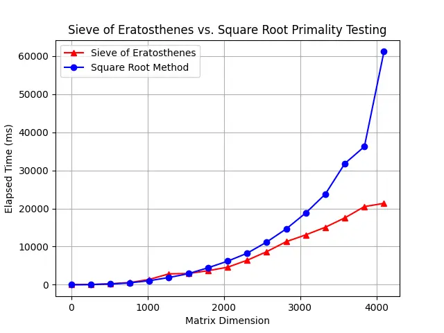
Is the theoretical speed up worth the increased space and code complexity? In the case of this Ulam spiral visualization tool, yes. The graph below compares the runtime of GenerateUlamSpiral() using the Sieve of Eratosthenes versus the Square Root method for primality testing. The graph shows dimensions in the range $[0, 4096]$. The plotted dimension values are at increments of $256$. The y-axis shows GenerateUlamSpiral()’s runtime. To minimize the effect of system delays on runtime measurements, the graph shows the average of $10$ samples at each dimension value.

As the dimension value increases, you can see the two lines start to diverge. That $0.5$ difference in the exponent has a significant effect on runtime even with small values of $N$!

Visualization

There’s a couple of different approaches you could take to visualizing the spiral. Generating a square, grayscale image is one of the simplest strategies. Each pixel in the image represents a cell in the Ulam Spiral matrix. You can color composite numbers’ pixels white and prime numbers’ pixels black. The output is an image with the expected diagonal, vertical, and horizontal lines characteristic of the Ulam Spiral.

The Boost Generic Image Library provides all the tools you need to write a Ulam Spiral to a grayscale PNG:

void WriteLatticeToPng(const std::string& filename,
                       const ulam::SquareLattice& ulam_mat) {
  boost::gil::gray8_image_t img(ulam_mat.size(), ulam_mat.size());

  auto output_view = boost::gil::view(img);
  for (int row = 0; row < output_view.height(); ++row) {
    for (int col = 0; col < output_view.width(); ++col) {
      /* Prime numbers are output as black pixels whereas composite numbers are
       * output as white pixels. */
      if (ulam_mat[row][col]) {
        output_view(col, row) = boost::gil::gray8_pixel_t(0);
      } else {
        output_view(col, row) = boost::gil::gray8_pixel_t(255);
      }
    }
  }

  boost::gil::write_view(filename, boost::gil::const_view(img),
                         boost::gil::png_tag{});
}

Below is 1024x1024 Ulam spiral grayscale image:

Wikipedia has a digestible explanation of the meaning behind the lines you see in the image.

Conclusion

Visualizing a Ulam spiral presents a number of challenges. Programmatically creating a square spiral through simulation is a nontrivial task. Similarly, deciding how to best test primality among the myriad of algorithms out there requires thought. Visualization is the least of your worries when libraries such as Boost’s GIL make writing images pixel-by-pixel a breeze. The end result is satisfying though. The lines in the Ulam spiral image are striking.

The complete project source is available on GitHub under ulam_spiral. Note, this project has since been rewritten in Rust. There were a number of benefits to the rewrite including support for more image formats, better unit testing, and benchmarking to name a few. The Rust version of the program uses the Sieve of Eratosthenes for primality checking. The performance of the Rust implementation is comparable to that of the original C++ implementation.

The Caesar Cipher (CC) is a classic symmetric key algorithm dating back to the time of Julius Caesar. If you are new to cryptography, the Caesar Cipher is a great first crypto algorithm to learn. This post will walk through the details of implementing a CC encrypt/decrypt function. You’ll then get a look at the internals of a CC code cracker.

Algorithm Description

There are four key ingredients to a Caesar Cipher:

• alphabet: The set of characters that may form an encrypted/decrypted message.
• plaintext: The secret message you’d like to transmit.
• ciphertext: The encrypted plaintext message.
• key: An integral shift applied to the characters in the plaintext message.

An example best illustrates how each of these components come together.

Suppose you want to send a secret message composed of only the lowercase English letters. You decide to use a Caesar Cipher to encrypt the plaintext “hello” using the key 14. To perform the encryption you map each character in the alphabet to an integer:

a	b	c	d	e	f	g	h	i	j	k	l	m	n	o	p	q	r	s	t	u	v	w	x	y	z
0	1	2	3	4	5	6	7	8	9	10	11	12	13	14	15	16	17	18	19	20	21	22	23	24	25

To perform the encryption, add the key to each characters’ integer representation modulo the size of the alphabet. For example, the letter “o” encrypts to $(14 + 14) \mod 26 = 2$ which according to the table is the letter “c.” The table below shows the encrypted form of “hello”:

h	e	l	l	o
v	s	z	z	c

“vszzc” is the ciphertext that you send to all your friends along with the key. To decrypt the message, your friends apply the same shifting process but in reverse. For example, the letter “c” in the ciphertext decrypts to $(2 - 14) \mod 26 = 14$ which maps to the letter “o.”

In general, the encryption and decryption formulas are:

$$E_n(x) = (x + n) \bmod |\Sigma|$$ $$D_n(x) = (x - n) \bmod |\Sigma|$$

where $x$ is the integer mapping of the encrypt/decrypt letter, $n$ is the key, and $|\Sigma|$ is the size of the alphabet.

Coding the Cipher

You can apply the CC encryption/decryption algorithm to any character set as long as you map each character to a unique integral value. In the world of computers and text, the ASCII character set is a perfect CC candidate. ASCII includes 128 characters each mapped to an integer in the range $[0, 127]$. The table below defines the ASCII character set. Only 95 out of 128 characters are printable.

Below is a C++ CC implementation that works with the ASCII alphabet:

RetCode AsciiCaesarCipher(std::istream &is, std::ostream &os, int shift) {
  if (!is) {
    return RetCode::kBadInputStream;
  }
  if (!os) {
    return RetCode::kBadOutputStream;
  }

  char curr = '\0';
  while (is.get(curr)) {
    curr = (static_cast<int>(curr) + shift) % kAsciiAlphabetSize;
    os << curr;
  }
  os.flush(); /* Flush the output stream just to be safe. */

  return RetCode::kSuccess;
}

Lets dissect this function starting with the function signature. AsciiCaesarCipher() takes three parameters: an input stream, an output stream, and a CC shift/key value. The input stream can be an open file (think std::ifstream), std::cin, or any other std::istream derived type. Similar to the input stream, the output stream can be an open file, std::cout, or some other std::ostream derived type. AsciiCaesarCipher() will output the result of the cipher to os. shift is the CC key as described in the previous section. AsciiCaesarCipher() returns a RetCode enum type:

enum class RetCode {
  kSuccess,
  kBadInputStream,
  kBadOutputStream,
};

The RetCode types are self explanatory.

AsciiCaesarCipher() reads characters out of the is stream one at a time. Each character has the CC shift applied. The shifted character gets output to os. The os.flush() call guarantees buffered data gets written to the recording medium. The same AsciiCaesarCipher() function can encrypt and decrypt ASCII text depending on the contents of is and the value of shift.

AsciiCaesarCipher() has a time complexity of $\mathcal{O}(N)$ where $N$ is the number of characters in the input stream. The space complexity is $\mathcal{O}(1)$. In reality, std::istream and std::ostream objects buffer data to reduce read/write overhead. The size of these buffers is implementation dependent though likely a small, constant size.

Cracking the Code

The Caesar Cipher isn’t immune to attack. Due to the small key space, one could perform a ciphertext only, brute force attack to recover the secret message. That would be tedious to do by hand. With the right algorithm, the computer can do the dirty work for you. Lets explore two attack techniques: a dictionary attack and a frequency analysis attack.

Dictionary Attack

A CC dictionary attack has you applying every possible shift to the ciphertext. The shift that produces the largest number of valid “words” is most likely the decryption key. To perform this attack, you need a dictionary of valid words.

Below is a C++ implementation of a CC dictionary attack. The algorithm assumes you’re working with the ASCII character set and that the message decrypts to regular English.

using WordSet = std::unordered_set<std::string>;
using KeyScoreMap = std::unordered_map<int, int>;

KeyScoreMap AsciiDictionaryAttack(std::istream& is, std::istream& dict_is) {
  WordSet dictionary = LoadDictionary(dict_is);
  KeyScoreMap scores;
  char curr = '\0';
  char tmp = '\0';
  std::string words[cipher::kAsciiAlphabetSize];
  while (is.get(curr)) {
    for (int shift = 0; shift < cipher::kAsciiAlphabetSize; ++shift) {
      /* Perform the Caesar Cipher shift. */
      tmp = (static_cast<int>(curr) + shift) % cipher::kAsciiAlphabetSize;

      if (std::isalnum(tmp)) { /* Add a char to the word at this shift. */
        words[shift] += std::tolower(tmp);
      } else if (!words[shift].empty() &&
                 std::isspace(tmp)) { /* Found complete word. */
        if (dictionary.count(words[shift])) {
          scores[shift]++;
        }
        words[shift].clear();
      }
    }
  }

  /* Check for the trailing words. */
  for (int shift = 0; shift < cipher::kAsciiAlphabetSize; ++shift) {
    if (dictionary.count(words[shift])) {
      scores[shift]++;
    }
  }
  return scores;
}

There’s a lot to talk about here. Lets start with the types WordSet and KeyScoreMap. WordSet is a set of strings representing the most popular English words in lowercase form. Why a set? Using a set, you can determine whether a string is an English word with an average time complexity of $\mathcal{O}(1)$.

KeyScoreMap is a map data structure. The map’s keys are CC shift/key values in the range $[0, 127]$. The map’s values are a tally of the number of English words seen when applying the corresponding shift key to the input stream.

AsciiDictionaryAttack() processes the input stream character by character. You apply each shift to the current input character. If following a shift the character is alphanumeric, then that character gets buffered in a string representing a candidate word. Otherwise, when a shift results in whitespace, the algorithm assumes a complete word proceeded the whitespace. In this case, if the word at the current shift value is an English word, the shift’s English word tally in scores gets incremented.

The output of AsciiDictionaryAttack() is a map with shift/key values and their scores. The key value with the highest score is the one you use to decrypt the ciphertext. It’s possible that two or more keys have the same score. In this case, apply all keys to find which makes most sense. The longer the input ciphertext is, the more likely you are to get an exact key match.

Frequency Analysis Attack

The frequency analysis attack depends on knowledge of the distribution of the ASCII characters in the English language. You take the ciphertext and apply all possible shifts to it. You then take a tally of the frequency of the characters in each translation as a percent value. The shift that produces the distribution closest to the expected distribution is the decryption key.

How do you know the distribution of ASCII characters in English? Someone has already done the hard part. The linked project analyzes the Reuters-21578 corpus to produce a table of ASCII frequencies. Note, some characters aren’t included in the table. You can assume the missing ASCII characters have a frequency of 0.

How do you compare distributions? There are a number of ways. One method is to treat the frequency distribution as a vector. In this case, the vector has 128 dimensions (one per ASCII character) where each dimension is a frequency represented as a percent value. You can compute the Manhattan Distance between two vectors to get a measure of how similar they are. The formula looks like this:

$$D = \sum_{i=0}^{127} |e_i - a_i|$$

where $e_i$ is the expected percent frequency of the ASCII character corresponding to $i$ in the English language. $a_i$ is the actual frequency of the character as measured in the ciphertext. The shift that produces the smallest distance value is the decryption key.

Lets look at the code:

using CharFrequencies = std::array<double, cipher::kAsciiAlphabetSize>;
using CharFrequencyArray =
    std::array<CharFrequencies, cipher::kAsciiAlphabetSize>;

KeyScoreMap AsciiFrequencyAnalysisAttack(std::istream& is) {
  CharFrequencyArray freqs;
  char curr = '\0';
  int tmp = 0;
  double num_chars = 0;
  while (is.get(curr)) {
    for (int shift = 0; shift < cipher::kAsciiAlphabetSize; ++shift) {
      /* Perform the Caesar Cipher shift. */
      tmp = (static_cast<int>(curr) + shift) % cipher::kAsciiAlphabetSize;

      /* Tally the shifted char. */
      freqs[shift][tmp]++;
    }
    num_chars++;
  }

  /* Calculate the percent frequency of each char. */
  for (auto& table : freqs) {
    for (double& val : table) {
      val /= num_chars;
    }
  }

  return FindMinDistShifts(freqs);
}

AsciiFrequencyAnalysisAttack() uses the CharFrequencyArray type to store the frequency distribution of each shift. The algorithm loops over the characters in the input stream and applies the CC to each character. The shifted character gets tallied in the corresponding frequency table. num_chars tracks the total number of characters in the ciphertext. num_chars comes into play in the final loop where the frequency counts get converted to a percentage.

FindMinDistShifts() finds the distribution with the smallest distance from the expected distribution using the Manhattan Distance metric previously described. The resulting KeyScoreMap will only have one shift key with a value set to one. The shift key with a value of one is the decryption key.

Lets look at an example. Suppose you encrypted this article using the key 42. Running the ciphertext through AsciiFrequencyAnalysisAttack() will return a KeyScoreMap with the following contents:

Key	Val
0	0
…	0
86	1
…	0
127	0

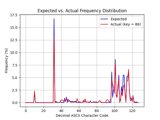
The results of AsciiFrequencyAnalysisAttack() suggests the decryption key is 86. The plot below shows the expected ASCII frequency distribution versus the frequency distribution of the ciphertext post decryption using the key 86.

The distributions match up well. If you were to decrypt using the key 86, you would indeed get the correct plaintext! Why is the decryption key 86 and not 42? Recall that to decrypt you take the negative of the encryption key modulo the size of the alphabet. In this case, $-42 \mod 128 = 86$.

Conclusion

The Caesar Cipher is a classic symmetric key crypto algorithm. The CC worked well in ancient times but doesn’t hold up so well in the age of computers. You can crack any CC code using a dictionary or frequency analysis attack. Neither attack is trivial. In the case of the dictionary attack, you need a valid dictionary to perform look ups on. The frequency analysis attack depends on knowledge of the expected distribution of alphabet characters. Regardless of its utility, the Caesar Cipher remains a fun algorithm to explore.

The complete project source is available on GitHub under caesar_cipher. Note, this project has since been rewritten in Rust. The Rust version of the project includes more testing but is otherwise a straight port of the C++.

This post includes the notes made while reading the book titled “Linux Kernel Development” by Robert Love.

Getting Started

The following are key differences between userspace application development and Linux kernel development:

• No access to the C library or C headers. There are versions of certain libc functions included in the kernel under lib/.
• The kernel uses GNU C. Kernel code follows ISO C99 and relies on some of GCC’s compiler extensions.
• The kernel lacks memory protection you might be use to in userspace. For example, illegal memory accesses in kernel code often leads to a fatal “oops” message.
• Kernel code can’t perform floating point operations (not in a straightforward way).
• The kernel has a small, fixed-size stack. The stack is usually about 2-4 pages with a page typically being 4k on 32-bit systems or 8k on 64-bit systems.
• Synchronization and concurrency is always an issue. This is due to async interrupts, preemption, and SMP support.
• Portability is important. Kernel developers segregate architecture specific code. General kernel code makes no assumptions about word size, page size, etc.

Processes

• In a Linux system using init, all processes all children of the init process with PID 1.
• Processes and threads are one and the same in Linux.
• The task_struct represents a process descriptor.
• Under the hood, the clone() function constructs a process or thread.
• The clone() function takes arguments which specify what process attributes get copied from the parent.
• When cloning, not all process data gets copied right away. Linux implements copy-on-write meaning pages aren’t copied until the parent or child process have written to them and therefore each need a separate copy. Linux does a trick where after cloning the child, it lets the child to run first. This makes it so if the child calls exec() to load a new program into its address space, it will do so immediately avoiding the situation where the parent runs, writes to one or more pages triggering a copy, and then the child runs exec() meaning that copy was for nothing.
• The current macro acquires the task_struct of the running process. current’s implementation varies from platform to platform with some systems storing the process descriptor in a register and others, like x86, placing it at the bottom of the process’s stack.
• Terminating a process doesn’t necessarily mean its gone. Terminated processes enter a zombie state. Once the process’s parent acknowledges the return code of the terminated child process, then the child process gets reaped.
• Zombie processes whose with a terminated parent are automatically re-parented. In the worst case they’re made direct children of the init process and then released.

Process Scheduling

• Linux supports multiple scheduling algorithms via its scheduling classes.
• The big schedule() function selects the next task to run by running the highest priority scheduler class with a runnable task.
• The O(1) scheduler and Completely Fair Schedule (CFS) scheduler are the most well known scheduling algorithms in the kernel.
• nice values are a measure of how nice a process is to the others. nice values range from -19 to 20. A lower value means a process is less nice. The less nice a process is the higher priority it has and vice versa. The default nice value in Linux is 0.
• CFS is the dominant scheduling algorithm. Also known as SCHED_OTHER.
• CFS is unique in that it optimizes for fairness by giving processes a proportion of the CPU’s time. That is, there is no hardcoded timeslice (other than a lower bound on the smallest amount of time any process could be allocated).
• CFS has two key parameters: target latency and minimum granularity. Target latency is an estimate of the infinitely small duration of time each process would get in an ideal system. Minimum granularity is a floor that’s set on the timeslice since in a real system you can’t have infinitely small timeslices.
• The nice values weight the proportion of CPU time each process gets. Each process runs for a “timeslice” proportional to its weight divided by the total weight of all runnable threads. See page 50-51 for an explanation of the benefit.
• At a high level, CFS tracks each process’s virtual runtime (that is, the amount of time a process has spent running. A red-black tree stores the vruntimes (that is, a height balanced binary search tree). The process chosen to run next is the process with the smallest vruntime (that is, the leftmost process in the tree). Instead of incurring a $\\mathcal{O}(logn)$ cost to retrieve this process, the kernel caches the left most node.
• sched_entity is the structure used by the kernel to account for a process’s scheduling. sched_entity is a field in the process descriptor task_struct.
• The vruntime is a time in nanoseconds weighted by the number of runnable processes.
• A context switch involves two things.
  • Switching the memory mapping context meaning swapping one processes pages for another. *
  • Switching the CPU context meaning one or more registers need the process info of the process being now set to run. Both of these steps are platform specific!
• need_resched is a per process flag that tells the kernel whether its time to switch processes. It’s checked on a return to userspace after a system call or after an interrupt gets serviced.
• The Linux kernel is preemptible. The kernel will only preempt kernel tasks if they don’t hold a lock. A task that doesn’t hold a lock is reentrant. Kernel preemption can occur:
  • When an interrupt handler exits, before returning to kernel-space.
  • When kernel code becomes preemptible again.
  • If a task in the kernel explicitly calls schedule().
  • If a task in the kernel blocks (which results in a call to schedule()).
• Page 65 gives a overview of how real-time priorities merge with nice values. Real-time priorities range from [0, 99]. Blended in are nice values which go from [100, 139].

System Calls

• System calls are the only interface to the kernel provided to userspace.
• The kernel maintains a system call table. The table is architecture specific. If you add a new syscall, you have to add it to each architecture’s syscall table!
• When a userspace application makes a system call, an exception gets triggered and the system call handler gets executed. The syscall handler is architecture specific. It will typically read the syscall code and parameters directly from CPU registers (means the caller loaded the registers up before trapping). A syscall return value also gets sent back via a specific register.
• System calls must be careful to validate all userspace parameters. Use the copy_from/to_user() when reading/writing data between spaces. They both block! Run the capability() method beforehand to check that the user has the right permissions to do what they’d like to do.
• It’s rare to add a new system call. Prefer exposing kernel info using files in sysfs or appropriate drivers with read()/write() implemented.

Kernel Data Structures

• The kernel includes linked lists, queues, maps, and binary trees for use by the developers. No need to write your own.
• The linked list provided is a circular doubly linked list. The struct list_head type gets embedded in a structure of your own. Then, a head node gets created using LIST_HEAD macros, finally you use the list manipulation functions and macros to add/remove/iterate.
• You can implement a queue or stack using the list API.
• Queues called kfifo are actually pretty vanilla and work much like you would expect in say C++.
• The maps are special. They’re like std::map in that the data gets sorted by key. Keys are always UIDs. The values in the map are void pointers. Under the hood, the map gets implemented using a balanced search tree of some sort.
• The tree structure provided by the kernel is the red-black self balanced BST. If using this structure, you have to handle search and insertion yourself! Look up examples cause it ain’t trivial.

Interrupts and Interrupt Handlers

• Interrupts are signals generated by hardware routed to the processor. The processor signals the kernel so that it may service the interrupt. Interrupts have a number assigned to them and a interrupt service routine that’s registered in the kernel to service specific IRQ numbers.
• Interrupts execute in an “atomic” context. Blocking isn’t allowed in an ISR. A interrupt can interrupt another executing interrupt!
• Interrupts get split into top and bottom halves. The top half does time-critical work. It’s meant to be quick and do just enough to service the HW and then return control to the kernel/process that was previously running. The bottom half is responsible for the actual processing of the received data and does the heavy lifting.
• request_irq() is the function used to register a interrupt handler. Interrupt handlers register from within the corresponding device driver. Interrupts are often shared. You enable interrupt sharing with the IRQF_SHARED flag.
• Interrupt handlers in Linux don’t need to be reentrant. When an IRQ line is gets serviced by a handler, that line gets masked out by the processor meaning another interrupt of that type can’t come in over the line.
• Interrupt handlers return IRQ_NONE or IRQ_HANDLED. IRQ_NONE gets returned when the interrupt handler detects an interrupt for which its device wasn’t the originator. IRQ_HANDLED gets returned if the interrupt handler was correctly invoked, and its device did indeed cause the interrupt. Most modern day devices provide a means for a driver to check whether the received interrupt was theirs. If it wasn’t, the ISR returns IRQ_NONE.
• Interrupt handlers can’t sleep/block!
• Interrupt handlers historically shared their stack with the interrupted process. Nowadays, the interrupt handlers have their own stack that’s one page in size.
• You can enable/disable interrupts on the current processor. This is typically done to support synchronization. Use local_irq_save() and local_irq_restore(). You must call these functions in the same stack frame (that is, within the same function)!
• You can disable an IRQ number for the entire system. You usually do this to configure a device. These are usually found in legacy ISA devices. Newer PCI devices share interrupts. Disabling interrupts for all devices on a line is not a good idea.

Bottom Halves and Deferring Work

• The reason for deferring work to a bottom half is in large part to reduce the amount of time the system is operating without interrupts. When an interrupt gets serviced, interrupts on that line get disabled across all CPUs. Worse yet, interrupt handlers can disable all interrupts on the local processor plus the interrupt of interest on all processors. Separating interrupt handling into two halves minimizes system latency.
• When to perform tasks in the upper half:
  • If the work is time sensitive, perform it in the interrupt handler.
  • If the work relates to the hardware, perform it in the interrupt handler.
  • If the work needs to guarantee that another interrupt (particularly the same interrupt) doesn’t interrupt it, perform it in the interrupt handler.
  • For everything else, consider performing the work in the bottom half.
• The bottom half facilities provided by the kernel are softirqs/tasklets and workqueues.
• softirqs are statically allocated bottom halves that can run on any CPU simultaneously.
• Tasklets are flexible, dynamically created bottom halves built on top of softirqs. Two different tasklets can run concurrently on different processors, but two of the same type of tasklet can’t run simultaneously. Note tasklets have nothing to do with tasks/processes!
• Workqueues use kthreads under the hood and run in process context. Use workqueues if you need the ability to block/sleep.
• Prefer softirqs for performance critical applications. They take more care to implement because they can run concurrently. You also must register them statically.
• Tasklets are more common for bottom half handling. Use a softirq only if you want the bottom half to run on more than one processor simultaneously and are ready to likely deal with per processor variables and what that entails.
• The kernel enforces a limit of 32 registered softirqs. In reality, only about 9 of those 32 softirqs are in use today. The others are reserves and can be taken by a programmer looking to implement a new softirq.
• A softirq never preempts another softirq. The only event that can preempt a softirq is an interrupt handler. In fact, softirqs get processed in sequence in the do_irq() function.
• Pending softirqs get checked for and executed in the following places:
  • In the return from hardware interrupt code path.
  • In the ksoftirqd kernel thread.
  • In any code that explicitly checks for and executes pending softirqs, such as the networking subsystem.
• Linux builds tasklets on top of the softirq system. The softirq flags differentiate between high and low priority tasklets. If the do_softirq() function finds a pending HI_SOFTIRQ or TASKLET_SOFTIRQ, then it will call the associated softirq action which happens to be one of tasklet_action() or tasklet_hi_action(). Either function will iterate over all their tasklets executing them only if the tasklet isn’t running on another processor. Tasklets with differing types can run concurrently!
• Tasklets can’t sleep/block.
• Tasklets run with interrupts enabled so be careful if you share data with an interrupt handler.
• If the system gets overloaded with softirqs, the kernel will spawn softirqd/n threads where n is the processor number. Idle CPUs will be able to service the softirqs.
• Work queues defer work as well. The most critical thing is that work queue tasks execute in a process context and can sleep/block.
• Work queues typically use generic kernel threads called worker threads. Worker threads have the label event/n where n is the CPU number.
• Work queues create a kernel thread on your behalf.
• Normal driver writers have two choices. First, do you need a schedulable entity to perform your deferred work? Do you need to sleep for any reason? Then work queues are your only option. Otherwise, use tasklets. Only if scalability becomes a concern do you investigate softirqs.
• Bottom halves can get disabled using the local_bh_enable/disable() functions.
• Bottom halve disabling usually comes up when process context code and bottom half code share data. You’ll need to disable bottom half processing and acquire a lock before accessing the shared data.

An Introduction to Kernel Synchronization

• The kernel provides facilities that support atomic variables.
• The kernel provides various forms of locks that protect a critical section.
• Concurrency is the root of all evil. There’s technically two types of concurrency: pseudo and true. Pseudo concurrency is when two processes/tasks get interleaved (perhaps on a single processor) creating the effect of unprotected, concurrent access. True concurrency is when processes/tasks run simultaneously on separate processors and access shared data.
• The kernel has many causes of concurrency:
  • Interrupts: An interrupt can occur asynchronously at almost any time, interrupting the current executing code.
  • Softirqs and tasklets: The kernel can raise or schedule a softirq or tasklet at almost any time, interrupting the current executing code.
  • Kernel preemption: Because the kernel is preemptive, one task in the kernel can preempt another.
  • Sleeping and synchronization with userspace: A task in the kernel can sleep and thus invoke the scheduler, resulting in the running of a new process.
  • Symmetrical Multiprocessing: Two or more processors can execute kernel code at exactly the same time.
• Code that’s safe from concurrent access from an interrupt handler is interrupt-safe.
• Code that’s safe from concurrency on symmetrical multiprocessing machines is SMP-safe.
• Code that’s safe from concurrency with kernel preemption is preempt-safe.
• Deadlock either self deadlock (double locking) or the ABBA deadlock is a real problem. The solution is to acquire resources with a fixed order and document that order.
• Lock contention can ruin performance. You need to balance how coarse/fine locking code is. Doing so can lend itself to making your code more scalable.

Kernel Synchronization Methods

• The kernel offers the atomic_t and atomic64_t types along with a series of inlined functions that initialize, increment, decrement, etc. the values.
• Each architecture guarantees the atomic_t type.
• The atomic64_t is only implemented by 64-bit architectures and should be avoided unless writing architecture specific code that relies on 64-bit operations.
• Atomic, bitwise operations are also provided. The bitwise ops work on raw memory or pointers directly.
• There are non-atomic versions of the bitwise operations as well. If you don’t have a requirement for atomicity, you should use the non-atomic versions because they’re faster.
• The kernel implements the classic busy waiting locks: spinlocks.
• Spinlocks are the only locks that you can use in interrupt handlers since they don’t cause the thread to sleep.
• When using a lock in an interrupt handler, one must disable interrupts. The spinlock interface in the kernel provides convenience functions that lock/unlock the lock and saves/restores the interrupt context. This prevents the double acquire deadlock from occurring.
• Because a bottom half might preempt process context code, if data gets shared between a BH process context, you must protect the data in process context with both a lock and the disabling of bottom halves.
• Because an interrupt handler might preempt a BH, if data gets shared between the two, you must both obtain a lock and disable interrupts.
• With Reader-Writer spinlocks, one or more readers to concurrently access shared data. When the writer acquires the lock, the writer gives exclusive access and the readers wait.
• Readers have priority in RW spinlocks! That is, it’s possible to starve the writer with enough readers!
• The kernel implements counting semaphores. A semaphore with a count of 1 is a binary semaphore (AKA mutex).
• When downing a semaphore, prefer down_interruptible() because the down() function will make the waiting task be in the TASK_UNINTERRUPTIBLE state which is likely not ideal.
• RW semaphores similar to the RW spinlocks are available. The RW semaphores place waiting tasks in an uninterruptible sleep!
• The kernel implements the mutex locking mechanism. You can think of the mutex as something separate from the binary semaphore previously mentioned.
• Unlike the semaphore, you can only unlock a mutex from the context in which you locked it. The kernel mutex doesn’t support recursive locking.
• There’s a special completion variable type. Completion variables make it possible to signal between threads when an event has occurred. They’re a lightweight alternative to semaphores.
• Sequential locks are RW locks that give preference to the writer. That is, the readers can never starve the writers.
• You can enable/disable preemption. See pages 201-202 for the reasoning.

Timers and Time Management

• The hardware implements a system timer whose frequency relates to a digital clock, CPU frequency, etc. When the timer goes off, a interrupt gets sent to the kernel.
• The kernel knows the preprogrammed tick rate so it knows the time between two successive timer interrupts. This is a tick and is equal to $\frac{1}{tickrate}$.
• The kernel uses this tick to track both wall clock time and system uptime.
• The timer interrupt performs the following tasks. Note some of these are executed every tick others every $N$ ticks:
  • Update the system uptime.
  • Update the time of day.
  • On an SMP system, ensuring balance in the scheduler runqueues and, if unbalanced, balancing them.
  • Running any dynamic timers that have expired.
  • Update resource usage and processor time statistics.
• Tick rate is in units of HZ. Never hardcode the tick rate, use the kernel provided APIs for accessing the value.
• Pros of a higher tick rate:
  • The timer interrupt has a higher resolution and, consequently, all timed events have a higher resolution.
  • The accuracy of timed events improves.
  • System calls such as poll() and select() that optionally employ a timeout execute with improved precision.
  • Measurements, such as resource usage or system uptime, get recorded with a finer resolution.
  • Process preemption occurs more accurately.
• Cons of a higher tickrate:
  • Increased power consumption.
  • Potential cache thrashing.
  • Increased overhead from the timer interrupt handler getting triggered.
• The global variable jiffies holds the number of ticks that have occurred since system boot.
• jiffies prototypes to unsigned long volatile jiffies. On 32-bit architectures it’s 32-bits and 64-bits on 64-bit architectures.
• You have to be cautious of the fact that the jiffies value may wrap around! To avoid issues with wrapping, using the kernel provided macros when comparing to jiffies:
  • time_after(unknown, known)
  • time_before(unknown, known)
  • time_after_eq(unknown, known)
  • time_before_eq(unknown, known)
• Architectures provide two pieces of HW for timekeeping: the system timer and the real-time clock (RTC).
• The RTC is a nonvolatile device for storing the system time. The RTC continues to track time even when the system is off by way of a small battery.
• On boot, the kernel reads the RTC value into the xtime variable. This initializes the wall time.
• The system timer’s key job is to provide a source of timer interrupts. What drive’s the system timer is platform dependent. Some system timer’s are programmable to specific rates.
• The timer interrupt has two parts: architecture dependent and independent routines.
• The architecture dependent routine gets registered as the ISR. Its tasking is platform specific. That said, they all do share some common functions:
  • Obtain the xtime_lock lock, which protects access to jiffies_64 and wall time value, xtime.
  • Acknowledge or reset the system timer as required.
  • Periodically save the updated wall time to the RTC.
  • Call the architecture-independent timer routine, tick_periodic().
• The architecture independent routine, tick_periodic(), performs much more work:
  • Increment the jiffies_64 count by one.
  • Update the resource usages, such as consumed system and user time, for the currently running process.
  • Run any dynamic timers that have expired.
  • Execute scheduler_tick().
  • Update the wall time, which gets stored in xtime.
  • Calculate the infamous load average.
• See page 222 for a description of how to use the timer API.
• Always use mod_timer() to update an active/inactive timer. If you don’t, races may occur.
• If deactivating an active timer, prefer del_timer_sync() over del_timer(). As the name suggests, the sync version waits for an associated timer handler running on another CPU to complete before returning. This is a blocking call so don’t use it from an interrupt context!
• Expired timers’ handler get run by the BH of the timer interrupt. Implemented as the softirq TIMER_SOFTIRQ.
• If you need a short delay (think microsecond delay) in a busy loop, use the udelay(), ndelay(), and mdelay() functions.
• A better solution is to call schedule_timeout() passing in the amount of time you would like to sleep in jiffies. The only guarantees here are that you don’t waste CPU time spinning and that your task will sleep at least as many jiffies as requested. Only call this function from a process context.

Memory Management

• The MMU deals with memory in terms of pages.
• The page struct tracks all physical pages in the system. It describes physical memory but not its contents. The goal is to indicate to the kernel whether a page is free. If a page is note free, the kernel can query the structure’s fields to know who owns it:
  • userspace processes
  • dynamically allocated kernel data
  • static kernel code
  • etc.
• The kernel instantiates a page struct per physical page. It’s a tiny bit wasteful of memory.
• Memory divides into zones. Below are four of the most popular zones:
  • ZONE_DMA: This zone contains pages that can undergo DMA.
  • ZONE_DMA32: LIke ZONE_DMA, this zone contains pages that can undergo DMA. Unlike ZONE_DMA, only 32-bit devices can access these pages. On some architectures, this zone is a larger subset of memory.
  • ZONE_NORMAL: This zone contains normal mapped pages.
  • ZONE_HIGHMEM: This zone contains “high memory,” which are pages not permanently mapped into the kernel’s address space.
• The kernel attempts to allocate memory from the appropriate zone. That said, if memory constrained, the kernel can pull memory from different zones. However, the kernel will never grab pages from two separate zones to satisfy a single request.
• Which zones are available is architecture dependent. Some architectures have only ZONE_DMA and ZONE_NORMAL because they can address the entire physical address space. Others like x86-32 have all four.
• struct page* alloc_pages(gfp_t gfp_mask, unsigned int order) is the kernel API for acquiring a list of $2^{order}$ contiguous pages.
• You can call the void* page_address(struct page* page) API to get the logical address of a page.
• Use unsigned long get_zeroed_page(unsigned int gfp_mask) to get the address of a single, zeroed out page.
• Table 12.2 shows all the low-level page allocation functions.
• There’s analogous page free functions for returning the pages that were acquired.
• Note, page allocation may fail. Try to allocate pages early and always check for allocation failure.
• The low-level page allocation functions only make sense to use if you need page sized chunks of memory.
• kmalloc()/kfree() is appropriate for allocating/freeing byte sized chunks of memory. It behaves much like malloc()/free(). The only difference is the added gfp_t flags parameter which controls how allocation.
• gfp stands for get free pages.
• gfp flags fall into three categories:
  • Action Modifiers: Specify how the kernel allocates the memory.
  • Zone Modifiers: Specify which zone the memory will come from.
  • Types: Acts as a combination of action and zone flags. There’s a couple of these like, GFP_KERNEL which define and OR of one or more action and zone flags.
• You only want to deal with type flags. Table 12.6 on Pg. 241 shows the available type flags and their description.
• vmalloc() acquires logically contiguous memory. It’s not typical that one uses vmalloc() due to its performance overhead or the need by the HW that memory acquired be physically contiguous. The function can sleep so it may only call it from a process context. Note, kmalloc() provides both physically and logically contiguous memory!
• The slab layer acts as a generic data structure-caching layer. It builds on the concept of free-lists where programmers maintain one or more lists of containing structures of commonly dynamically allocated types.
• The slab layer divides different objects into groups called caches, each of a different type of object. There’s once cache per object type.
• Caches divide into slabs where each slab is one or more contiguous pages of memory.
• Each slab contains some number of objects of a specific type.
• Slabs are always in one of three states: full, empty, or partial. Partial slabs allocations happen before empty slab allocations.
• You can make your own slab allocator caches for some custom object type.
• Kernel stack size is customizable ranging from 1 to 2 pages of memory.
• In the past, interrupt handlers shared the running process’s stack. Nowadays, each interrupt handler gets its own page for a stack. This requires one page per processor.
• Stack overflows occur silently in the kernel. There is no check for it! Keep stack usage to a few hundred bytes. If you need more memory, dynamically allocate it!
• You can map a limited number of pages from high memory into the kernel’s address space. Do this sparingly. Blocking and nonblocking interfaces are available to do this mapping.
• The kernel provides interfaces for statically and dynamically allocating per-cpu variables. There are also APIs for getting/putting CPU variables that take care of any preemption issues.
• Never access a per-cpu variable across CPUs without some form of synchronization.
• Reasons to use per-cpu variables:
  • A reduction in locking requirements.
  • Improved cache behavior.
  • Enable access from interrupt and process context.
• Never sleep when working on a per-cpu variable!

The Virtual Filesystem

• The virtual filesystem (VFS) provides an interface by which one can use the usual system calls (for example, open(), write(), read(), etc.) to interact with myriad filesystems and devices. You never need to rewrite or recompile your program to work with ext2 versus ext4 filesystem thanks to the VFS.
• The VFS provides an abstraction. New filesystems must implement the VFS interface and use its data structures to “plugin” to the kernel.
• An inode or index node is just file metadata (for example, time of creation, owner, permissions, etc.).
• The VFS has a OOP architecture.
• The four primary object types of the VFS are:
  • superblock: Represents a specific mounted filesystem.
  • inode: Represents a specific file.
  • dentry: Represents a directory entry which is any component of a path (file or directory).
  • file: Represents an open file associated with a process.
• Each object has a *_operations structure which contains function pointers to specific operations on that object. The kernel provides a default implementation of a few of the methods. However, filesystem developers likely have to implement their own operations so that they “make sense” for their specific use case.
• Each filesystem implements the superblock object and uses it to store information describing that specific filesystem (AKA the filesystem control block).
• An inode represents each file on the filesystem, but the inodes object constructs in memory only as files get accessed. inodes can even represent special files like pipes, block devices, or char devices (but only one at a time).
• Unix inodes typically separate file data from its control information (for example, metadata).
• dentries get cached in the dcache. When a file path is first resolved, each component in the path is a dentry and gets cached in the dcache.
• dentry accesses exhibit temporal and spatial locality similar to program instructions and data. This makes the dcache effective in reducing file access times.
• dentries associate with an inode. The dcache serves as an icache since actively used inodes get pinned along with their dentry in the dcache.

The Block I/O Layer

• Block devices are hardware devices distinguished by the random access of fixed sized chunks of data.
• Block devices mount a filesystem. As a user, you interact with the block device via the filesystem.
• In contrast to block devices, char devices provide a sequential stream of char data. It doesn’t make sense to random access the data of a char device. That’s where the block device comes in.
• The smallest addressable unit on a block device is a sector. Typically a power of two with the most common size being 512 bytes.
• Although a device is addressable at the sector level, the kernel usually operates on blocks. The block is an abstraction of the filesystem and can be only be a multiple of the sector size, no larger than the page size, and must be a power of two.
• Each block gets its own buffer. The buffer is an in memory representation of the block. Each block gets a buffer head which is essentially a descriptor describing the block (which device owns the buffer, page info, etc.).
• The buffer head’s bh_state flag (see page 292) tells one the state of the buffer. Within bh_state there’s a number of bits reserved for driver authors to use.
• Block buffers benefit from storing block data on a page. That said the block buffer approach is a bit wasteful since you need multiple buffers/block heads to for example write large amounts of data.
• The bio struct is the block buffer’s replacement. The struct represents block IO operations that are active as a list of segments. A segment is a chunk of a buffer that’s contiguous in memory. Segments make scatter/gather IO possible in the kernel. See page 295 for a illustration.
• With the bio struct, the buffer is now represented as an array of bio_vec structs where each bio_vec includes a page, offset, and length. The full array of bio_vec structs is the buffer.
• The way to think of all this is that each block IO request gets represented as a bio struct. Each request is one or more blocks stored in the array of bio_vec structures of the bio struct (these are the segments). As the block IO layer submits request, the bi_index gets updated to point to the next bio_vec struct.
• Buffer heads are still relevant. They’re required for describing the device’s blocks.
• Block devices maintain request queues to store their pending block IO requests. The filesystem adds requests to the queue and dispatches them to the block device’s driver for processing.
• The kernel includes a block IO scheduler to merge and sort requests. The idea here is that IO performance would be terrible if requests were simply serviced in the order received. You want to reduce seek times and optimize the order in which requests are services. The IO schedule does the latter by virtualizing the block devices similar to how the process scheduler virtualizes the CPU.
• The IO scheduler works by managing a block device’s request queue. It decides the order of requests in the queue at what time each request gets dispatched to the block device. It optimizes on seek to improve *global throughput**. That is, the IO scheduler doesn’t care much for fairness.
• The IO scheduler performs two primary actions to minimize seeks:
  • Merging is the coalescing of two or more request into one.
  • Sorting refers to how the IO scheduler keeps requests in the queue sorted sector wise so that all seeking activity moves as close to sequential as possible.
• There are many different IO scheduler algorithms supported by the kernel:
  • The Linus Elevator: Performs both the merge and sort operations. Uses an insertion sort to maintain the sector ordering of the request queue and will merge adjacent sectors on insertion. There’s an issue with requests starving with this algorithm if requests cluster around one area of the disk leaving the far off requests to starve.
  • The Deadline IO Scheduler: This algorithm uses three queues: a queue sorted on sector just like the previous one, a write FIFO, and read FIFO. The write/read FIFO queues are essentially sorted on time. Write request have an expiration of about 5 seconds into the future while read requests have an expiration delta of about 500 milliseconds. When the Deadline scheduler dispatches a request, it first checks if there is an expired request in one of the FIFO queues before issuing a request from the sorted queue. In this way, you avoid starvation. Also note the bias towards read requests. If you delay read requests significantly, application performance would degrade notably (imagine all the time spent blocking on read())!
  • The Anticipatory IO Scheduler: This algorithm is identical to the Deadline IO scheduler except there is an added heuristic: the anticipation heuristic. It’s meant to resolve the delay in write heavy systems that occasionally read. In the latter scenario with a Deadline IO scheduler, the seek head would bounce back and forth as infrequent reads would be immediately serviced triggering a long seek. The trick here is that after servicing a read request, the algorithm will wait for a configurable amount of time before returning to the previous request. This makes it such that if another read requests comes in during the wait, it can immediately get serviced with a reduction in the time spent seeking. The algorithm uses per process block IO statistics to improve its behavior over time. The algorithm avoids starvation, reduces read latency, and increases overall throughput through the reduction of seeks/seek time.
  • The Completely Fair Queueing IO Scheduler: This one’s a bit different than the rest. CFQ gives each process an IO request queue. The queue are serviced round robin. The number of requests consumed at each queue visit is configurable. CFQ works well with specific workloads particularly those associated with multimedia.
  • NOOP IO Scheduler: This algorithm does little more than insertion sort incoming request by sector size. Beyond that, it’s basically a FIFO algorithm. NOOP works well with block devices such as flash memory which have no overhead with seeking and thus don’t need all the bookkeeping and added overhead of the other algorithms.

Debugging

• Unsurprisingly, printk() is one of the key debug tools.
• printk() is robust in that you can call it anywhere and anytime within kernel code.
• printk() supports eight different log level macros. Use the one that’s appropriate for the situation (or example, if debugging, use KERN_DEBUG). You will need to set the console log level accordingly to see the messages in the kernel logs.
• A kernel oops occurs when the kernel encounters an error condition from which it can’t proceed/recover.
• The Oops message contains info such as the contents of CPU registers, a stack trace, and more.
• Sometimes the oops that’s printed isn’t decoded (that is, the stack trace is just a bunch of addresses). You can save the oops message in a text file. Then, using the ksymoops program, you can decode the oops message.
• In place of ksymoops shenanigans, you can enable CONFIG_KALLSYMS_ALL at kernel config time. This decodes the entire oops message at the cost of an increased kernel image (probably worth it unless you need a min size kernel image).
• In the “Kernel Hacking” section of the kernel config editor, you can enable many debug options. Enable as many as needed to solve your problem.
• The BUG_ON(condition) macro triggers an oops purposefully.
• panic() is another developer macro that will halt the kernel at the call site.
• dump_stack() will do what the name suggests. Useful with an added printk() message to give context to the dump.
• You can use the kgdb features of the kernel to run gdb on a live kernel. See the StarLabs article for the details.
• Git bisect is your friend when tracking down kernel bugs.

Portability

• One of the key goals of Linux is portability.
• The majority of the core/subsystem code in the kernel is portable/platform agnostic. Architecture specific code lives in arch/
• Some code must be platform specific. For example, context switch code for registers and address space switches are platform specific.
• The kernel has a number of APIs that each platform must implement. For example, each platform implements switch_to() and switch_mm().
• Architectures that support both 32 and 64-bit word sizes have their codebases tied together under one architecture. For example, x86 holds x86-32 and x86-64 platform code.
• The long type always has a size equal to the platform’s word size. Don’t assume the size of long to be 32-bits or 64-bits. Use the macro BITS_PER_WORD to compute word size portably.
• Only use opaque types such as pid_t and atomic_t as specified by their API. Never assume anything about their size or underlying type. Don’t convert opaque types to some C built-in type.
• Use the fixed size types when appropriate (for example, u32, s32, u8, s8, etc.). You can’t export the fixed size types to userspace. Instead, you must use the userspace friendly versions that prefixed with double underscores (for example, __u32).
• On a N-bit system, data should be (N/8) byte aligned. For example, a 32-bit system is usually 32/8 = 4 byte aligned. The bottom 3 bits of each address should be zero.
• Alignment is usually handled by the compiler and not a concern to the programmer. One place worth being aware of alignment is in structures where the compiler adds padding automatically to meet alignment requirements. Sometimes you can avoid the overhead of padding by re-arranging the members of the struct to meet padding requirements. The compiler will never reorder structure members on your behalf!
• If you have concerns over endianness and need to convert to/from the CPU ordering and LE/BE, use the kernel’s endianness conversion API.
• Never assume the frequency of the timer interrupt. Always use the HZ macro to compute an estimate for time.
• Never assume the page size. Use the PAGE_SIZE macro instead. If you need the number bits to left shift an address to derive its page number, use the PAGE_SHIFT macro.
• Always assume and program for an SMP/preempt/highmem system. This keeps you safe in any kernel/HW configuration.

Have you implemented a shared pointer class in C++? If you have, did you do it in an interview setting? You might be familiar with the STL shared_ptr and the fact that many implementations of shared_ptr use reference counting to manage the lifetime of a dynamically allocated object. That said, if you’ve never thought about or tried to actually implement the concept itself, doing so in an interview is a tall order. This article walks you through the implementation of an interview grade SharedPtr class.

How to Reference Count

When you think about implementing a shared pointer, what comes to mind? Wrapping the user’s pointer and counting how many SharedPtr objects point to the same location seems like a reasonable strategy. Here’s a first attempt at setting up this bookkeeping:

template <typename T>
class SharedPtr {
 public:
    ...
 private:
    T* data_;
    std::size_t ref_count_;
};

This declaration is mostly correct. The T* data_ member is right. You need a way of sharing and accessing the data. What better way than a pointer to the data. After all, a shared pointer is a lightweight wrapper around a raw pointer. The std::size_t ref_count_ variable seems like a good idea, however, it doesn’t work for ref counting. Why? What happens when you copy, assign, destroy, or call Reset() on a SharedPtr? In those instances, you need to decrement/increment the ref_count_. You can certainly update the ref_count_ in the object performing the operation. However, there’s no clear way to communicate the increment/decrement to all other SharedPtr instances wrapping the same data_ pointer.

What’s the trick? Change the declaration of ref_count_ to std::size_t* ref_count_. The ref count itself is a pointer that’s shared by all SharedPtr instances wrapping the same data_ pointer. The first SharedPtr to wrap data_ is responsible for allocating ref_count_. When ref_count_ hits 0, ref_count_ deallocates along with data_.

Lets work an example. Consider the code below:

void Nonsense() {
    SharedPtr<int> p1(new int(42));
    SharedPtr<int> p2 = p1;
}

How do p1 and p2 evolve from when you first enter the Nonsense() function’s scope until right before destruction? Try going line-by-line starting with the instantiation of p1:

                                 +------------+      +-----------------+
                                 |     P1     |      |   Main Memory   |
                                 +------------+      +-----------------+
SharedPtr<int> p1(new int(42));  |  data_     +----->| 42              |
                                 +------------+      +-----------------+
                                 | ref_count_ +----->| 1               |
                                 +------------+      +-----------------+

Nothing too crazy here. You wrap a pointer to the value 42. Your ref count points to a value of 1. What happens when you assign p1 to p2?

                         +------------+      +-----------------+
                         |     P1     |      |   Main Memory   |
                         +------------+      +-----------------+
                         | data_      +----->| 42              |<-+
                         +------------+      +-----------------+  |
                         | ref_count_ +----->| 2               |<-+-+
                         +------------+      +-----------------+  | |
SharedPtr<int> p2 = p1;                                           | |
                         +------------+                           | |
                         |     P2     |                           | |
                         +------------+                           | |
                         | data_      +---------------------------+ |
                         +------------+                             |
                         | ref_count_ +-----------------------------+
                         +------------+

Here the SharedPtr works its magic. Both p1 and p2 point to the same data in memory via a copy of the data_ pointer. You bookkeep ref_count_ during the assignment in p2. Specifically, *ref_count_ gets incremented from 1 to 2. The key thing to note is that even though the increment to ref_count_ came from the p2 object, p1 sees the change. Why? Because p1 and p2 point to the same area in memory containing the ref_count_ value.

The API

The SharedPtr API is similar in spirit to the STL’s shared_ptr:

template <typename T>
class SharedPtr {
 public:
  SharedPtr();
  explicit SharedPtr(T* data);
  ~SharedPtr();

  SharedPtr(const SharedPtr& sp);
  SharedPtr& operator=(SharedPtr rhs);
  SharedPtr(SharedPtr&& sp);
  SharedPtr& operator=(SharedPtr&& rhs);

  const T& operator*() const;
  T& operator*();

  bool Empty() const;
  std::size_t RefCount() const;
  void Reset(T* data);

  template <typename U>
  friend void Swap(SharedPtr<U>& a, SharedPtr<U>& b);
};

Here are the key features starting from the top:

• SharedPtr is a template class that wraps a pointer to any type T.
• You can default construct SharedPtr.
• Included is a constructor that takes ownership of a raw pointer.
• You can copy/move construct and assign SharedPtr objects.
• The dereference operator gets overloaded.
• One can verify whether the pointer is empty or NULL.
• One can access the reference count.
• You can wrap another dynamically allocated object without leaking memory to the originally wrapped object via a Reset() call.

You’ll notice a friend Swap() method towards the end of the declaration. Swap() implements the copy-and-swap idiom. Swap() simplifies the implementation of copy assignment and move construction/assignment. More on that later.

The Basics

Construction, dereferencing, ref counting, and empty/NULL checks have a straightforward implementation:

template <typename T>
SharedPtr<T>::SharedPtr() : data_(nullptr), ref_count_(nullptr) {}

template <typename T>
SharedPtr<T>::SharedPtr(T* data)
    : data_(data), ref_count_(new std::size_t(1)) {}

template <typename T>
bool SharedPtr<T>::Empty() const { return (!data_ && !ref_count_); }

template <typename T>
std::size_t SharedPtr<T>::RefCount() const {
  if (Empty()) {
    throw std::runtime_error("cannot return ref count of NULL SharedPtr");
  }
  return *ref_count_;
}

template <typename T>
const T& SharedPtr<T>::operator*() const {
  if (Empty()) {
    throw std::runtime_error("cannot dereference NULL SharedPtr");
  }
  return *data_;
}

template <typename T>
T& SharedPtr<T>::operator*() {
  if (Empty()) {
    throw std::runtime_error("cannot dereference NULL SharedPtr");
  }
  return *data_;
}

This implementation throws std::runtime_error when a user attempts to access the reference count or data of an uninitialized SharedPtr. This was a decision made to make the class more test friendly and avoid any undefined behavior. It’s also worth mentioning that the call to new in the nondefault constructor has the potential to throw std::bad_alloc along with introducing the overhead of an allocation. Since you’re already using exceptions for error handling and wrapping dynamically allocated objects, the latter “issues” are probably negligible in most codebases opting to use SharedPtr.

Reference Counter Bookkeeping

The core of the SharedPtr implementation is how the ref_count_ member gets updated. That is, you need to manage ref_count_ increment/decrement and guarantee the wrapped resource gets released when ref_count_ reaches 0. To do this right, you can enumerate all the places ref_count_ gets updated.

ref_count_ gets incremented:

• On nondefault construction.
• On copy construction.

ref_count_ gets decremented:

• On destruction.
• On copy or move assignment.
• After a call to Reset().

Decrement happens more often and has the added overhead of checking whether the ref_count_ reached 0. In the interest of not duplicating the decrement and ref count check code, I implemented a utility method: DecrementRefCount():

template <typename T>
void SharedPtr<T>::DecrementRefCount() {
  if (Empty()) {
    return;
  }

  *ref_count_ -= 1;
  if (0 == *ref_count_) {
    delete data_;
    delete ref_count_;
    data_ = nullptr;
    ref_count_ = nullptr;
  }
}

DecrementRefCount() makes the implementation of the remaining API methods relatively straightforward:

template <typename T>
SharedPtr<T>::~SharedPtr() {
  DecrementRefCount();
  data_ = nullptr;
  ref_count_ = nullptr;
}

template <typename T>
SharedPtr<T>::SharedPtr(const SharedPtr<T>& sp)
    : data_(sp.data_), ref_count_(sp.ref_count_) {
  *ref_count_ += 1;
}

template <typename T>
SharedPtr<T>& SharedPtr<T>::operator=(SharedPtr rhs) {
  DecrementRefCount();
  Swap(*this, rhs);

  return *this;
}

template <typename T>
SharedPtr<T>::SharedPtr(SharedPtr&& sp) : SharedPtr<T>() {
  Swap(*this, sp);
}

template <typename T>
SharedPtr<T>& SharedPtr<T>::operator=(SharedPtr&& rhs) {
  DecrementRefCount();

  Swap(*this, rhs);

  return *this;
}

template <typename T>
void SharedPtr<T>::Reset(T* data) {
  DecrementRefCount();

  data_ = data;
  ref_count_ = new std::size_t(1);
}

The copy-and-swap idiom helps implement copy/move assignment and the move constructor. Critical to the use of this idiom is the implementation of a Swap() function that can swap the state of two SharedPtr objects:

template <typename U>
friend void Swap(SharedPtr<U>& a, SharedPtr<U>& b) {
  using std::swap;
  swap(a.data_, b.data_);
  swap(a.ref_count_, b.ref_count_);
}

The post linked at the end of this article explains the rationale behind the idiom and dives into the gritty details.

Conclusion

Creating a SharedPtr class is an interesting problem with some fun edge cases and quirks. It’s not too hard to understand why someone would want to ask a question like this. Getting a proper implementation requires some diagramming and careful bookkeeping. Questions around error handling and memory management also come up. Now whether it’s a good question for a 30min interview is another story.

The complete project source with build instructions, usage, etc. is available on GitHub under shared_ptr.

This article gives an overview of how to setup a Linux kernel development environment that leverages QEMU. Why should you bother with this setup? Here are the highlights:

• Make changes to core kernel code or modules without the risk of loading buggy kernel code onto real hardware.
• Up the speed of the edit, build, run cycle while developing kernel code.
• The ability to test code across different architectures (for example, aarch64, x86_64, etc.).

What’s QEMU? According to Wikipedia:

QEMU (Quick Emulator) is a free and open-source emulator. It emulates a computer’s processor through dynamic binary translation and provides a set of different hardware and device models for the machine, enabling it to run a variety of guest operating systems. It can interoperate with Kernel-based Virtual Machine (KVM) to run virtual machines at near-native speed. QEMU can also do emulation for user-level processes, allowing applications compiled for one architecture to run on another.

QEMU has three main operating modes:

• User-mode Emulation: Run a single program compiled with a different instruction set than that of the host machine.
• System Emulation: Emulate an entire computer system, including peripherals. This is what most people mean when they say “virtual machine.”
• Hypervisor Support: As the name suggests, this mode has QEMU leverage a hypervisor (for example, Linux Kernel-based Virtual Machine or KVM). This is the most performant option.

This article demos hypervisor support mode. Below is an illustration showing the intended setup:

graph LR
    subgraph PC["PC"]
        Host["Host OS"] <-->|SSH| Guest["Guest OS"]
    end

The goal is to run a guest OS on your host machine. The guest OS will run a Linux distro of your choice along with your custom kernel. From within the guest, you got all the comforts of a full fledged Linux system and can poke and prod without any fear. The SSH connection makes it easy to transfer some files to/from the guest.

{{}}

Install QEMU and OpenSSH

First, download and install QEMU and OpenSSH on the host machine.

The following install commands work on a Fedora 38 machine. If you are using another distro, adjust the package manager and package names!

sudo dnf install qemu qemu-image openssh

Create an Image

You’ll need a virtual disk image to install the guest OS. You can create an image using qemu-img:

qemu-img create -f raw <MY_IMAGE> 4G

You can change 4G to whatever size in gigabytes you can afford. Worth mentioning is the alternative qcow2 image format. While slower than a raw formatted image, the qcow2 image size increases during VM usage. You set a limit in gigabytes on the size of the qcow2 image during creation.

Install a Distro

The world is your oyster when it comes to distros. It doesn’t matter what distro you use. Arch Linux is a solid choice since a base install is pretty bare bones. Plus, you can tell everyone you use Arch. Download the latest ISO and follow the steps below to get started with the install.

You’ll first want to load the Arch installer by telling QEMU to boot off an emulated CD-ROM with your Arch ISO on it:

qemu-system-x86_64 \
    -enable-kvm \
    -cdrom <ARCH_ISO> \
    -boot order=d \
    -drive file=<MY_IMAGE>,format=raw \
    -m 4G

Lets take a moment to breakdown these options:

Option	Description
-enable-kvm	Enable hypervisor support using the Linux KVM.
-cdrom	Points to what image will be inserted into our emulated CD slot.
-boot	Tell QEMU we want to boot from CD-ROM.
-drive	Specifies a drive on the system. We tell QEMU about our previously created image file and its format.
-m	Tell QEMU the size of RAM. The more the better.

A quick side note on KVM support. It’s possible though unlikely your PC doesn’t have KVM support. If you try to run the command and QEMU complains about a lack of KVM support try the following:

• Verify the host processor has virtualization enabled. Run lscpu | grep Virtualization. If you are on an Intel machine with virtualization enabled, the output will be Virtualization: VT-x. If your output doesn’t match, enable virtualization in the BIOS menu.
• Some distros require your user be part of a KVM group. You can add yourself to such a group using the command: sudo usermod -aG kvm $USER. Replace kvm with name of the KVM group on your system.
• Most mainstream distros ship a Linux kernel with KVM features enabled. If that isn’t the case for you, then you may have to tweak your kernel’s command line args or install a kernel with kvm_guest.config applied.

After running the qemu-system-x86_64 command, you will see a QEMU window that has the Arch Installer running:

You can now go RTFM (that is, the Arch wiki installation guide). The alternative is to use the archinstaller script to do the heavy lifting for you. The following Youtube video has all the details on how to do just that (you can skip to the 2:16 mark):

{{< youtube d5rquFPwh-Y >}}

Building the Kernel

This section assumes you know how to build and configure a Linux kernel. There are plenty of videos and tutorials online if you need a refresher.

Below are the commands for preparing a kernel meant to run in a QEMU VM:

make O=/my/build/dir defconfig
make O=/my/build/dir kvm_guest.config
make O=/my/build/dir nconfig # Optionally configure additional kernel params
make O=/my/build/dir -j$(nproc)

The only oddity is perhaps the addition of kvm_guest.config. Building this config enables a number of Kernel-based Virtual Machine (KVM) options allowing the kernel to boot as a KVM guest. Also, re-directing the output of the build using the O= option to make isn’t necessary but does keep your kernel source tree clean.

You can cross-compile the kernel for your architecture of choice. You can then run the appropriate qemu-system-* binary to emulate that architecture on the host. However, you can’t use the KVM features across platforms. For example, if you’re on an x86_64 host and cross compile and run a aarch64 VM, then you can’t leverage the -enable-kvm switch to enable KVM features. In this example, you would have to run QEMU in system emulation mode not hypervisor mode.

Boot the Virtual Machine

Moment of truth. Time to boot the VM. This bash script gives the QEMU incantation:

#!/bin/bash

DISK="kernel-dev-archlinux.img"
KERNEL="/home/ieg/dev/kernel/build/arch/x86/boot/bzImage"

qemu-system-x86_64 \
    -enable-kvm \
    -drive format=raw,file=$DISK \
    -m 4G \
    -nic user,hostfwd=tcp::2222-:22 \
    -serial stdio \
    -smp 4,sockets=1,cores=2,threads=2,maxcpus=4 \
    -kernel $KERNEL \
    -append "root=/dev/sda2 console=ttyS0,115200 rw" \
    -display none

Once again, this is command line soup. Lets look at what each switch is doing.

Option	Description
-enable-kvm	Enable hypervisor support using the Linux KVM.
-drive	Defines the virtual drive (AKA the disk image we previously created and installed our distro to).
-m	RAM size.
-nic	Setup net options. We specify user mode and setup port forwarding for SSH.
-serial	Redirect the virtual serial port. We redirect serial debug info to stdio.
-smp	Simulate an SMP system. I used lscpu to pass the config of my host system but you do not have to!
-kernel	Path to the kernel bzImage.
-append	This is the kernel commandline. We tell the kernel where the rootfs is and setup the console.
-display	Selects the type of display to use. The none arg makes it so no video output is displayed.

After running the script, you will see a VM terminal. You can verify your kernel is running via the uname -a command:

If the uname command prints your kernel version, you are all set! Just one last thing left to do: setup SSH.

SSH Setup

While you won’t be developing directly on the VM, you might want to transfer a number of files between the host and VM (for example, loadable modules). SSH and the scp utility are perfect for that.

SSH’ing as root

If you don’t mind using the root account in the VM, follow these steps to login as root on the VM over SSH:

1. Login to the VM as root.
2. Install openssh:

pacman -Syu openssh

3. Edit /etc/ssh/sshd_config and uncomment PermitRootLogin yes.
4. Stop and then enable the sshd service:

systemctl stop sshd
systemctl enable sshd

5. From the host machine, SSH to the VM:

ssh -p 2222 root@localhost

SSH’ing as a User

If instead of using the root user you would like to login as my_user, follow these steps:

1. Login to the VM as root. Optionally, if my_user has sudo privileges, login as my_user.
2. Install openssh:

pacman -Syu openssh

3. Enable the sshd service:

systemctl enable sshd

4. From the host machine, SSH to the VM:

ssh -p 2222 my_user@localhost

Conclusion

If you do a lot of kernel development, a workflow that uses QEMU may be for you. Using a VM makes it easier to make and deploy kernel changes when compared to most target hardware setups. Plus, there’s the added benefit that if/when you yeet the system, you can patch your changes and just fire up a fresh VM. Also, keep in mind that QEMU can do a lot more than what’s shown here. Definitely take a look at other QEMU tutorials and experiment a bit.

This post includes the notes made while reading “Linux Driver Development for Embedded Processors” by Alberto Liberal de los Rios. Notes weren’t taken for every chapter so keep in mind that the book actually covers more topics than what’s shown here.

If you are considering buying the book, you might want to checkout this review before buying.

Character Drivers

• There are three primary ways of creating a character driver:
  • Statically create the device.
  • Use the devtmpfs approach with create_class()/create_device().
  • Use the misc framework.
• Block and character drivers have both a major and minor number.
• The major number maps a device to a driver. Every driver has a major number assigned to it.
• A driver can have one or more minor numbers. The minor numbers’ meaning is managed by the driver implementation.
• You can edit the /linux/drivers/char/[Makefile|KConfig] to add an entry for loading your custom char driver.
• Don’t statically assign major numbers. Prefer to use the devtmpfs method instead. devtmpfs is a virtual filesystem that mounts to /dev. Basically, using the create_class()/create_device() methods, your driver will automatically have an entry in /dev. Requires CONFIG_DEVTMPFS_MOUNT be enabled in the kernel config. Note, the latter option doesn’t work if booting using an initramfs.
• There is a limit on the number of major numbers and it wastes RAM to keep them around. If you have a simple char device, it’s preferable to use the misc framework. All misc devices have a major of 10 but the minor can be dynamically or statically assigned. This approach is good for devices with just one minor (they do something basic).
• sysfs is another virtual filesystem mounted to /sys. sysfs has a structure and contents that describe the hardware onboard the system. Device classes, including those created using devtmpfs create* calls, appear under /sys/class.
• udev is a userspace daemon that listens for uevents and makes use of the info in sysfs. Admins can configure udev rules to name devices, setup symlinks, react to certain events (for example, device plugin) etc.
• “What Populates the sys and dev Directories”.

Platform Drivers

• Platform drivers are drivers that bound to devices defined in the device tree (DT).
• Platform drivers bind to their device node in the DT using the compatible string. The driver sets up the compatible string using struct of_device_id and the MODULE_DEVICE_TABLE macro.
• Linux a has a core platform driver subsystem which will scan the DT and bind a device to the driver using the compatible string. On binding, the platform driver ops trigger. Specifically probe() on initialization and remove() on exit.
• probe() performs the following functions:
  • Gets a pointer to a device structure as an argument (for example, struct pci_dev *, struct usb_dev *, struct platform_device *, struct i2c_client *, etc.).
  • Initializes the device, maps I/O memory, allocates buffers, registers interrupt handlers, timers, etc.
  • It registers the device to a specific framework (for example, network, misc, serial, input, industrial).
• Many pins are multifunction. Multifunction pins multiplex to a single function.
• Linux has a pinctrl subsystem for which board developers write pinctrl drivers specific to their hardware. Look at the kernel docs under linux/Documentation/devicetree/bindings/pinctrl/brcm,bcm2835-gpio.txt if you feel you need more info.
• Linux has a GPIO controller driver as well. There is an API for accessing and configuring GPIO pins called the GPIO descriptor consumer interface.
• GPIOs have the option to map to devices and functions in the device tree. The exact way to do it depends on the GPIO controller providing the GPIOs (see the device tree bindings for your controller). Reference page 143.
• GPIOs mapped to IRQs in the DT and then a driver can access that GPIO IRQ number to register interrupts on that IRQ.
• The UIO framework serves to implement the core of a driver from userspace. Below is summary of the pros/cons of a UIO driver:
  • Pros:
    • Easy to debug as debug tools are more available for application development.
    • User space services such as floating point are available.
    • Device access is efficient as there is no system call required.
    • The application API of Linux is stable.
    • You write the driver in any language.
  • Cons:
    • No access to the kernel frameworks and services.
    • You can’t handle interrupts in user space. You must handle interrupts in a kernel driver.
    • There is no predefined API to provide applications access to a device driver.
• Below is a summary of the pros/cons of kernel space drivers:
  • Pros:
    • Runs in kernel space in the highest privilege mode to allowing access to interrupts and hardware resources.
    • There are a lot of kernel services such that kernel space drivers can be designed for complex devices.
    • The kernel provides an API to user space allowing multiple applications to access a kernel space driver simultaneously.
  • Cons:
    • System call overhead to access drivers.
    • Challenging to debug.
    • Frequent kernel API changes. Kernel drivers built for one kernel version may not build for another.
• You can either use the generic UIO driver specified as uio-generic in the DT or write a custom platform driver that plugs into the UIO framework.
• UIO is especially handy for mapping device memory straight into the userspace and letting userspace do what it will with the device.
• Interrupt handling is a bit weird. Userspace can’t register or handle interrupts. The UIO driver must handle the interrupt. A userspace app can block waiting for an interrupt using read() or select().
• If you use the generic-uio driver you must also set the kernel boot arg uio_pdrv_genirq.of_id=generic-uio. The generic driver will magically map the reg field of the DT into memory so that your userspace app can access that memory using mmap().

I2C Devices

• There are three entities to consider: The I2C Bus, I2C Controller, and I2C Client.
  • The I2C Bus is a kernel framework for registering I2C controllers and provides an API that a I2C client can use to tx/rx data using the specific controller for that system.
  • The I2C Controller must define a transfer function used as a callback by the I2C bus driver. The I2C controller implements the details of the I2C controller onboard the SoM.
  • The I2C client is a driver for a specific I2C device. Think accelerometers, ADCs etc. It uses the I2C Bus API to tx/rx data.

Interrupts

• You can leverage GPIOs as interrupt pins. You must configure the GPIOs and interrupt controller in the DT to use GPIOs as interrupt pins. The “interrupt” property defines a GPIO interrupt.
• Interrupts split into a time-critical top half that runs in interrupt context and an optional bottom half which runs at some later time in process context. The bottom half does the heavy lifting.
• To achieve the interrupt split, use deferred work. Deferred work takes many forms:
  • Threaded IRQs
  • Tasklets
  • Workqueues
• Tasklets may only run on a single CPU concurrently. Tasklets execute in an interrupt context so no blocking/sleeping is okay.
• A typical flow in the kernel is ALL ISRs -> ALL TASKLETS -> Process Threads (both kernel and user)
• ISRs run at essentially infinite priority and mask the interrupt they’re servicing. You want ISRs not to block or sleep for that reason.
• Tasklets build off of softirqs. If there are too many softrirqs or softirq processing is taking to long, the kernel will create ksoftirqd/N threads to schedule the processing of the softirqs.
• Threaded IRQs are means of specifying both a top half and bottom half routine for interrupt handling. The top half runs in interrupt context, the bottom half runs as a kernel thread in process context.
• Workqueues add work to a global “events” workqueue maintained by the kernel. From the ISR, you can schedule work (that is, kickoff a thread to service the interrupt data at some later time).
• You can also spawn your own kthreads (not recommended).
• Timers are an option for drivers. Timers build off of the softirq system. You register a timer ISR with your timer and then set it. Subsequently, your timer ISR gets called on timer expiration, there you can do some work and schedule another timer. You define timer expiration using jiffies.
• A jiffy is a time value that starts from 0 on boot and increments by 1 every system timer tick. The “jiffies” macro is available as a global. You can use the HZ macro (a mirror of CONFIG_HZ) to convert jiffies to time or vice versa. There’s also plenty of helper macros in the kernel that do said conversion.
• Waitqueues are a means of deferring work as well. You setup a waitqueue with some function registered. From within an ISR or elsewhere in the driver code, you can kick off the work waiting in the queue. The scheduler schedules the work at some later time and will execute in process context. There are two types of waitqueues: interruptible and non-interruptible. Interruptible means that a signal can wake the thread. Waitqueues also have an option for setting expiry timers.