A classic weekend programming project is to write a Chip8 emulator. Chip8 refers to an interpreter for a simple instruction set architecture (ISA) that saw use in the 1970s COMSAC VIP microcomputer. You could program the VIP’s CDP1802 processor by writing Chip8 instructions: hexadecimal opcodes that resemble machine code but are more high-level.

This article will discuss a number of sticking points you might encounter when implementing your own Chip8 emulator. Note, the issues discussed here are language agnostic. At the end of the article, you’ll find a link to a Rust implementation of a Chip8 emulator that can serve as a more complete reference.

The Many Forms of Chip8

To start, you’ll want to get your hands on a Chip8 specification. The fun part is that there are many different specifications since Chip8 has seen an evolution over the years.

COMSAC VIP Specification

The most common specification is the original one for the COMSAC VIP. The original specification includes the following components (the listing below comes directly from Tobias’ Chip8 Guide):

• Memory: Chip8 has direct access to up to 4 kilobytes of RAM.
• Display: 64x32 monochrome pixel display.
• A program counter which points at the current instruction in memory.
• One 16-bit index register called “I” which points at locations in memory.
• A stack for 16-bit addresses. The stack plays a role in the implementation of subroutines/functions and returning from them.
• An 8-bit delay timer which decrements at a rate of 60 Hz until it reaches 0.
• An 8-bit sound timer which functions like the delay timer, but which also gives off a beeping sound as long as it’s not 0.
• Sixteen 8-bit general purpose variable registers numbered 0 through F called V0 through VF.

The instruction set consists of 35 instructions:

Instruction	Description
0NNN	Execute machine language subroutine at address NNN
00E0	Clear the screen
00EE	Return from a subroutine
1NNN	Jump to address NNN
2NNN	Execute subroutine starting at address NNN
3XNN	Skip the following instruction if the value of register VX equals NN
4XNN	Skip the following instruction if the value of register VX is not equal to NN
5XY0	Skip the following instruction if the value of register VX is equal to the value of register VY
6XNN	Store number NN in register VX
7XNN	Add the value NN to register VX
8XY0	Store the value of register VY in register VX
8XY1	Set VX to VX OR VY
8XY2	Set VX to VX AND VY
8XY3	Set VX to VX XOR VY
8XY4	Add the value of register VY to register VX Set VF to 01 if a carry occurs Set VF to 00 if a carry does not occur
8XY5	Subtract the value of register VY from register VX Set VF to 00 if a borrow occurs Set VF to 01 if a borrow does not occur
8XY6	Store the value of register VY shifted right one bit in register VX Set register VF to the least significant bit prior to the shift VY is unchanged
8XY7	Set register VX to the value of VY minus VX Set VF to 00 if a borrow occurs Set VF to 01 if a borrow does not occur
8XYE	Store the value of register VY shifted left one bit in register VX Set register VF to the most significant bit prior to the shift VY is unchanged
9XY0	Skip the following instruction if the value of register VX is not equal to the value of register VY
ANNN	Store memory address NNN in register I
BNNN	Jump to address NNN + V0
CXNN	Set VX to a random number with a mask of NN
DXYN	Draw a sprite at position VX, VY with N bytes of sprite data starting at the address stored in I Set VF to 01 if any set pixels are changed to unset, and 00 otherwise
EX9E	Skip the following instruction if the key corresponding to the hex value currently stored in register VX is pressed
EXA1	Skip the following instruction if the key corresponding to the hex value currently stored in register VX is not pressed
FX07	Store the current value of the delay timer in register VX
FX0A	Wait for a keypress and store the result in register VX
FX15	Set the delay timer to the value of register VX
FX18	Set the sound timer to the value of register VX
FX1E	Add the value stored in register VX to register I
FX29	Set I to the memory address of the sprite data corresponding to the hexadecimal digit stored in register VX
FX33	Store the binary-coded decimal equivalent of the value stored in register VX at addresses I, I + 1, and I + 2
FX55	Store the values of registers V0 to VX inclusive in memory starting at address I I is set to I + X + 1 after operation
FX65	Fill registers V0 to VX inclusive with the values stored in memory starting at address I I is set to I + X + 1 after operation

This article will focus on this version of the spec.

SuperChip8

SuperChip8 is a 1990s extension of the original Chip8 specification. The extension focuses on improving graphic and display capabilities. Here’s a summary of the changes:

• Higher Resolution: SuperChip8 supports a 128x64 pixel display mode.
• High Resolution Toggle: New instructions 00FF and 00FE enable and disable the high-resolution graphics mode, respectively.
• Scrolling: SuperChip8 adds instructions for scrolling the display: 00CN (scroll down), 00FB (scroll right), and 00FC (scroll left).
• Larger Sprites: The existing DXYN instruction in SuperChip8 draws 16x16 sprites when N is 0.
• Larger Fonts: SuperChip8 includes a larger hexadecimal font, 8 pixels wide and 10 pixels tall, available via the FX30 instruction.
• Exit Instruction: 00FD lets a program exit the interpreter.
• Flag Register Operations: FX75 and FX85 instructions let you save and load values to and from user flag registers, providing a form of persistent storage.

XO-Chip

XO-Chip is a modern extension of the Chip8 specification developed by John Earnest in 2014. Below is a excerpt from the “official” chip-8 docs):

XO-Chip supports audio and 64 kilobytes of memory, which is usable mainly for graphics and audio (addressable only by I). It also has one extra buffer (“plane”) of display memory, which works identical to the regular one. Planes display on top of each other, and they can have different colors. You can draw illuminated pixels in both planes in another color. Clear, draw and scroll instructions will only affect the currently selected planes.

XO-Chip is mainly supported by John Earnest’s own Octo assembler, which supports “macros” for comparison operators but which assembles down to regular Chip8 bytecode instead of dedicated instructions.

Instructions

Most Chip8 instructions have a side effect. Instructions alter the state of the registers, graphic display, timers, or memory. To ease instruction implementation, make data structures representing each of these components. Give these structures methods for read-only access and methods for mutating the state. It makes the code easier to read and removes much of the repetition. See state.rs for examples.

Probably the best tip (lifted directly from Tobias’ Guide) for handling Chip8 instructions is to decode the 16-bit value into a structure like DecodedInstruction shown below:

/// Internal structure for holding parsed components of a CHIP-8 instruction.
///
/// This structure breaks down a 16-bit instruction word into its constituent
/// parts for easier access during instruction execution.
struct DecodedInstruction {
    /// First nibble. Represents the operation code.
    opcode: u8,
    /// Second nibble. Used to look up one of the 16 registers.
    x: usize,
    /// Third nibble. Used to look up one of the 16 registers.
    y: usize,
    /// Fourth nibble. A 4-bit number.
    n: u8,
    /// The second byte (third and fourth nibbles). An 8-bit immediate number.
    nn: u8,
    /// The second, third, and fourth nibbles. A 12-bit immediate address.
    nnn: Address,
}

When you process an instruction, you can first decode it into a DecodedInstruction which gives easy access to the components of the instruction. During execution, you can access the desired component without performing bitwise operations to read the values.

The final and most crucial tip regarding instructions is to make sure to read the specification two to three times! The extra 2-3 minutes spent reading the spec will save you hours of debugging later.

The Run Loop

Now the Chip8 emulator run loop is for the most part straightforward. The emulator executes at 60 Hz. This means the display and timers update at a rate of 60 times per second.

How many instructions run per second? Now that’s the tricky part. The original Chip8 processor ran at 1 MHz. That doesn’t tell you much since the Chip8 instructions take a different number of cycles to run. Many Chip8 implementers target an Instructions Per Second (IPS) rate of 700. This seems to work best for most Chip8 games. Ideally, you want to make the IPS value configurable so that the User can adjust it as needed.

Below is some pseudocode illustrating the run loop:

FRAMES_PER_SEC = 60
IPS = 700
INSTRUCTIONS_PER_FRAME = IPS / FRAMES_PER_SEC

last_time = 0
loop:
    curr_time = get_current_time()

    if curr_time - last_time >= 1 / FRAMES_PER_SEC:
        for _ in range(INSTRUCTIONS_PER_FRAME):
            fetch_instruction()
            decode_instruction()
            execute_instruction()

        update_timers()
        render_display()

        last_time = curr_time

Testing Your Emulator

If you’re like most programmers, your emulator will have bugs. Luckily, there are a number of test ROMs that you can run to verify your implementation.

This is where Timendus’s Chip8 Test Suite saves the day. Timendus provides ROMs that test drawing, flag handling, quirks, and more. See the project’s README for instructions along with helpful screenshots illustrating what to expect for each test.

Conclusion

Writing a Chip8 emulator is an excellent introduction to emulation development. The simplicity of the Chip8 instruction set makes it approachable for beginners, while implementation quirks and timing considerations provide enough depth to keep things interesting. Start with the original COSMAC VIP specification, implement instructions methodically using the DecodedInstruction pattern, and use test ROMs like Timendus’s suite to verify your work. Once complete, you’ll have gained valuable experience in instruction decoding, memory management, and graphics rendering that applies to more complex emulation projects.

The complete project source is available on GitHub under chip8.

This is a quick and dirty guide to setting up a local LLM. You’ll see how to run the Qwen2.5-Code-3B-Instruct model on your local machine using vllm. You’ll then setup the CodeCompanion plugin in NeoVim for interacting with the model directly from your editor.

vLLM Installation and Server Setup

Step one is to install the vllm CLI utility:

python -m venv local-llm
source local-llm/bin/activate
pip install vllm

The vllm tool will download and standup a local server for the model. Take note of what hardware you have available (RAM, CPU, GPU/VRAM) and then browse models at hugginface.co. This example kicks off a Qwen2.5-Code-3B-Instruct model server:

vllm serve --model Qwen2.5-Code-3B-Instruct

The command will take a few minutes to run as it downloads the model and sets up the server. A successful run will look like this:

Starting vLLM API server 0 on http://0.0.0.0:8000
...
INFO: Started server process [5853]
INFO: Waiting for application startup.
INFO: Application startup complete.
INFO: 172.22.117.26:436999 - "GET /v1/models HTTP/1.1" 200 OK

The server is now ready to accept requests.

NeoVim Setup with CodeCompanion

CodeCompanion is one of many plugins meant to assists in integrating LLMs with NeoVim. CodeCompanion groups LLM configuration via adapters. The plugin includes many default adapters for popular LLMs. However, it doesn’t have an adapter for the Qwen model.

Below is a Lazy plugin configuration for CodeCompanion that adds an adapter for the Qwen model.

{
    "olimorris/code-companion.nvim",
    lazy = false,
    depedendencies = {
        "nvim-lua/plenary.nvim",
        "nvim-treesitter/nvim-treesitter",
    },
    config = {
        adapters = {
            qwen = function()
                return require("codecompanion.adapters").extend("openai_compatible", {
                    env = {
                        url = "http://localhost:8000",
                        chat_url = "/v1/chat/completions",
                        models_endpoint = "/v1/models",
                    },
                })
            end,
        },
        strategies = {
            chat = {
                adapter = "qwen",
            },
            inline = {
                adapter = "qwen",
            },
            cmd = {
                adapter = "qwen",
            },
        },
    }
}

Since the Qwen model is OpenAI compatible, you can inherit from the openai_compatible adapter and extend it with the necessary configuration.

The plugin requires the markdown and markdown_inline Tree-sitter parsers. Install them both with :TSInstall markdown markdown_inline. You can also improve your experience by installing a number of additional plugins. See Additional Plugins for more information.

Further Reading

For CodeCompanion usage instructions, refer to the user guide. In general, CodeCompanion provides a chat interface for querying the LLM. There’s also support for inline prompting (that is, you highlight a section of code and ask the LLM for help).

For more information on vLLM (the library not the CLI utility), checkout this RedHat article.

This post includes the notes made while reading the book “Code - The Hidden Language of Computer Hardware and Software 2nd Edition” by Charles Petzgold.

Chapter 2: Codes and Combinations

• Morse Code is a binary language. International Morse Code encodes up to 8 bits of information where each bit is either a dot or a dash.
• Dots and dashes are the written representation of Morse Code. The dot is a short signal, while the dash is a long signal. The length of the dash is three times that of the dot.
• As with all binary codes, each time you add a bit, you double the number of possible combinations.

Chapter 3: Braille and Binary Codes

• Braille is a type of binary code where 6 bits represent a character. The 6 bits arrange in a 3x2 grid, where each dot can be either raised or not raised. The 6 bits can represent 64 different characters.
• Though there are only 64 characters, Braille characters can have additional meanings based on their context.
• The number indicator marks the beginning of a sequence of numbers. The letter indicator terminates the number sequence. This is an example of a shift code.
• In Braille, the capital indicator capitalizes the letter that follows. The capital indicator is an example of an escape code. Escape codes change the meaning of the code that immediately follows.

Chapter 4: Anatomy of a Flashlight

• You can characterize electricity as the flow of electrons.
• In the flashlight example, the battery is the source of electricity. The flashlight bulb is the load. The switch is a control device that opens and closes the circuit.
• Batteries produce a chemical reaction that creates a flow of electrons. Chemical energy converts to electrical energy. Spare electrons appear on the anode side of the battery. The cathode side of the battery has a deficiency of electrons. Electrons would like to flow from the anode to the cathode.
• An electrical circuit provides a path for the flow of electrons from the anode to the cathode.
• Substances composed of atoms that bias towards shedding electrons are conductors. Copper, silver, and gold are good conductors.
• The opposite of conductance is resistance. Substances with high resistance are called insulators. Rubber, glass, and plastic are good insulators.
• Current ($I$) is the flow of electrons through a circuit.
• Voltage ($V$) is the difference in electric potential between two points in a circuit.
• Voltage is directly proportional to the amount of current flowing through a circuit. Current is inversely proportional to resistance. Also known as Ohm’s Law: $V = IR$.
• Power in Watts is the product of voltage and current: $P = IV$.

Chapter 5: Communicating Around Corners

• You can make a primitive telegraph by connecting two batteries, four wires, and two light bulbs.
• You can remove a wire from the circuit by using a common ground. Ground in this case means a connection to the Earth.
• The Earth acts a source of electrons. The electrons flow from the Earth, through the circuit, and into the positive terminal of the battery.
• American Wire Gauge (AWG) is a measure of wire thickness. The lower the number, the thicker the wire. The thicker the wire, the less resistance it has.
• When covering great distances, you need to use thicker wire or a higher voltage power supply.

Chapter 6: Logic with Switches

• George Boole invented Boolean algebra. Boolean algebra is a system of logic.
• You can describe boolean algebra in terms of sets. The usual set operators such as union, intersection, and complement apply as do the concepts of the universe and NULL set.
• Two switches wired in series are equivalent to an AND gate.
• Two switches wired in parallel are equivalent to an OR gate.
• You can configure switches and wires to form complex boolean expressions. A primitive form of a computer.

Chapter 7: Telegraphs and Relays

• The invention of the telegraph marks the beginning of modern communication. For the first time, people could communicate over long distances almost instantaneously.
• The telegraph key is a switch that opens and closes the circuit to send messages. The telegraph operator taps the key to send dots and dashes.
• The telegraph sounder is a device that converts the electrical signals from the telegraph key into audible sounds.
• One major impediment to the telegraph was the length of the wires needed to connect the telegraph stations. The longer the wire, the more resistance it has, and the weaker the signal.
• The invention of the relay solved the problem of long-distance telegraphy. A relay is an electrically operated switch that can amplify the signal.
• A relay consists of an electromagnet, a set of contacts, and a spring. When the electromagnet gets energized, it attracts the armature, which closes the contacts and completes the circuit.

Chapter 8: Relays and Gates

• Reduced to its essentials, a computer is a synthesis of Boolean algebra and electricity.
• The crucial components of a computer are the logic gates. Logic gates are electronic circuits that perform boolean operations.
• Like switches, you can connect relays in series or parallel as logic gates. You can combine logic gates to form more complex circuits.
• The switches control the input to the relays, and the relays control the output. The output of one relay can be the input to another relay.
• A normally open relay is a relay that’s open when the electromagnet isn’t energized. A normally closed relay is a relay that’s closed when the electromagnet isn’t energized.
• An inverter is a logic gate that reverses the input signal. In terms of relays, an inverter is a normally closed relay that opens when the electromagnet gets energized.
• There are six basic logic gates: AND, OR, NOT, NAND, NOR, and XOR.
• Additionally, you have buffers. A buffer is a logic gate that passes the input signal to the output without changing it. In real life circuits, sometimes output must serve as many inputs. That’s called fanout, and it can result in a lessening of the power available to each input. Buffers can help boost that power acting as a relay. You can also use buffers to delay a signal.
• From a NAND or NOR gate, you can create all other logic gates.
• The following are Demorgan’s Laws:
  • $\lnot A \land \lnot B = \lnot(A \lor B)$
  • $\lnot A \lor \lnot B = \lnot(A \land B)$
• Demorgan’s Laws are useful for simplifying boolean expressions.

Chapter 9: Our Ten Digits

• There are many possible number systems.
• Roman numerals were common before the introduction of the Hindu-Arabic numeral system. Key features that differentiate the Hindu-Arabic numeral system include:
  • The use of a zero to represent the absence of a value.
  • The positional notation, where the value of a digit depends on its position in the number.

Chapter 10: Alternative 10s

• By convention, humans work in a base 10 number system, also known as decimal.

• There are many other number systems, such as binary (base 2), octal (base 8), and hexadecimal (base 16).

• The formula for converting from any base to decimal is:

  $$d = \sum_{i=0}^{n} d_i \cdot b^i$$

  where $d$ is the decimal value, $d_i$ is the digit in base $b$, and $n$ is the position of the digit.

• Binary numbers unite arithmetic and electricity. Switches, wires, and light bulbs can all represent the binary digits 0 and 1, and with the addition of logic gates, you can manipulate these numbers.

Chapter 11: Bit by Bit by Bit

• The binary number system is the simplest number system possible.
• The bit, a binary digit, is the fundamental unit of information in computing.
• The meaning of a particular bit or collection of bits is always understood contextually.
• You can visualize binary codes in many ways. The example given is the Universal Product Code (UPC) barcode. The UPC barcode is a binary code that encodes information about a product. A slice of the barcode has black lines representing 1 and gaps representing 0. The thickness of the lines or gaps dictate the number of bits represented (up to 4 bits per line). In total, the UPC barcode encodes 95 bits of data.
• The UPC barcode also includes some error checking. The last digit is a checksum that verifies the integrity of the data. Each barcode includes a beginning, middle, and end guard pattern to help scanners identify faulty codes.
• Quick Response (QR) codes are another example of a binary code. QR codes can encode more information than UPC barcodes, including URLs and text. QR codes consist of black squares arranged on a white grid. The black squares represent 1s, and the white squares represent 0s. Most of the bits in a QR code are for error correction.

Chapter 12: Bytes and Hexadecimal

• Computers often group bits into a quantity called a word with the most common word size being 8 bits, also known as a byte.
• Modern computers typically use 32-bit or 64-bit words.
• The hexadecimal number system is a base 16 number system that uses the digits 0-9 and the letters A-F to represent values.
• You can group the digits in a binary number into sets of four to form a hexadecimal digit.

Chapter 13: From ASCII to Unicode

• Morse code is a variable bit-length code, meaning that different characters can have different numbers of bits. For example, the letter ‘E’ is a single dot (1 bit), while ‘Q’ is a dash followed by two dots (3 bits).
• Braille is a fixed-length code, meaning that each character has the same number of bits (6 bits).
• ASCII (American Standard Code for Information Interchange) is a character encoding standard that uses 7 bits to represent characters. ASCII can represent 128 different characters, including letters, digits, and control characters.
• ASCII includes 32 control characters that are not printable, such as the newline character and the tab character.
• ASCII is also known as plain text. ASCII data does not include any formatting information, such as font size or color.
• Extended ASCII is an 8-bit character encoding that includes additional characters beyond the standard ASCII set. Extended ASCII can represent 256 different characters.
• Extended ASCII can’t represent characters from all different languages and scripts.
• Unicode is a character encoding standard that can represent characters from many different languages and scripts. Unicode started as a 16-bit encoding.
• Unicode documents start with a Byte Order Mark to indicate endianness.
• Unicode has more recently extended to 21 bits, allowing it to represent over a million different characters.
• Unicode transformation formats (UTF) encode Unicode characters in a way that’s compatible with existing systems. The most common UTFs are UTF-8, UTF-16, and UTF-32.
• UTF-8 is the most widely used Unicode encoding. It uses 1 to 4 bytes to represent characters, depending on the character’s code point. How bytes are interpreted is complex enough that you should look this up for more details.

Chapter 14: Adding with Logic Gates

• The summation of two bits produces a sum bit and a carry bit.
• You create an XOR gate by passing the two inputs through both a OR gate and a NAND gate, and then passing the outputs through a AND gate:
• An XOR gate takes two input bits and produces a sum bit.
• An AND gate takes two input bits and produces a carry bit.
• You can combine XOR and AND gates to create a half adder, which adds two bits and produces a sum bit and a carry bit.
• A full adder is a circuit that adds three bits: two input bits and a carry bit from a previous addition. A full adder produces a sum bit and a carry bit. You can combine two half adders and an OR gate to create a full adder (see page 177).
• You can combine two 8 bit full adders to create a 16 bit adder (see page 182). You can combine multiple 16 bit adders to create larger adders.

Chapter 15: Is This For Real

• Relays and vacuum tubes were the first electronic components used in computers.
• You can build logic gates from vacuum tubes just like you can with relays.
• Relays suffer slow switching speeds and are susceptible to mechanical wear.
• Vacuum tubes are faster than relays but are larger, consume more power, generate more heat, and wear more often.
• The transition from relay technology to vacuum tube technology marked the transition from electromechanical computers to electronic computers.
• Von Neumann architecture is a design for a computer that uses a single memory space for both data and instructions. This architecture is the basis for most modern computers.
• You can control a semiconductors’ conductance by applying a voltage. This property makes them ideal for building logic gates and other electronic components.
• Semiconductor doping is the process of adding impurities to a semiconductor to change its electrical properties. The most common dopants are phosphorus and boron forming n-type and p-type semiconductors.
• You can make amplifiers out of semiconductors by sandwiching a p-type semiconductor between two n-type semiconductors. This is the basis for a NPN transistor, and the three pieces form the collector, base, and emitter.
• A small voltage on the base controls the flow of current between the collector and emitter.
• The transistor introduces solid-state electronics, which means transistors are built from solids, specifically semiconductors and most commonly silicon.
• Transistors require much less power, generate much less heat, and last longer than vacuum tubes.
• The invention of the integrated circuit (IC) allowed for the miniaturization of electronic components. An IC is a small chip that contains many transistors and other electronic components.
• The first ICs were usually packaged in dual in-line packages (DIPs).
• There are two families of ICs: transistor-transistor logic (TTL) and complementary metal-oxide-semiconductor (CMOS).
• TTL chips are faster but consume more power than CMOS chips. CMOS chips are slower but consume less power and are more tolerant to variations in voltages.
• One important fact to know about a particular integrated circuit is the propagation time, the time it takes for a change in the inputs to reflect in the output.
• You measure propagation time in nanoseconds.
• The timeline to keep in mind from this chapter is that logic gate components trended from relays, to vacuum tubes, to transistors, and then to integrated circuits.

Chapter 16: But What About Subtraction

• This chapter introduces two’s complement, a method for representing signed integers in binary.
• Two’s complement makes for easy addition and subtraction of signed integers using the same binary addition circuits previously discussed.
• To convert a positive integer to two’s complement, you simply represent it in binary. To convert a negative integer to two’s complement, you invert the bits of its positive representation and add 1.
• Since binary numbers have a fixed number of bits, you can only represent integers within a certain range. For example, with 8 bits, you can represent signed integers from -128 to 127 or unsigned integers from 0 to 255.
• There’s opportunity for overflow when adding or subtracting signed integers. The circuit on page 210 shows how to detect overflow in a two’s complement addition circuit.

Chapter 17: Feedback and Flip-Flops

• You can create an oscillator by connecting the output of an inverter to its input. The inverter will toggle its output between 0 and 1, creating a square wave.
• The period of an oscillator is the time it takes for the output to complete one cycle. The frequency is the number of cycles per second.
• The frequency of an oscillator is inversely proportional to its period. Usually, you measure frequency in Hertz.
• See page 221 for an illustration of a reset-set flip-flop.
• The next flip-flop type is the level triggered D-type flip-flop. The D stands for data. The D flip-flop captures the value of the data input when the clock signal is high and holds that value until the next clock cycle.
• A edge triggered D-type flip-flop captures the value of the data input on the rising or falling edge of the clock signal.
• You can make an edge triggered D-type flip-flop by combining two level triggered flip-flops (see page 229).
• If you combine an oscillator with a edge triggered D-type flip-flop, you can create a frequency divider. The output frequency is half the input frequency. See page 235 for an illustration of a frequency divider.
• Chained frequency dividers create a binary counter called a ripple counter.
• To find the frequency of the oscillator, you can let the ripple counter run for a certain number of cycles and then divide the number of cycles by the time it took to run them.
• You can augment a flip-flop with a clear and preset input. You never set both clear and preset at the same time.
• Having a clear input avoids the issue of the flip-flop being in an indeterminate state when powered on.
• With the preset input, you can set the flip-flop to a known state without waiting for the clock signal.

Chapter 18: Let’s Build a Clock

• Binary Coded Decimal (BCD) is a way of representing decimal numbers in binary. BCD uses 4 bits to represent each decimal digit, allowing you to represent decimal numbers from 0 to 9.
• It’s best to read the book to get an idea of how to build the clock. At a high level, you use a ripple counter to count each digit in the seconds, minutes, and hours. The output of the high digit’s counter is the input to the next counter. Additional circuitry makes it possible to display the hours in 12-hour format.
• Electrical current can only flow in one direction through a diode.
• A Light Emitting Diode (LED) is a diode that emits light when current flows through it.
• A diode matrix is a grid of diodes that displays characters or numbers. The diodes are in rows and columns, and you can turn on specific diodes to create a pattern.
• Diode matrices are technically a form of Read Only Memory (ROM).

Chapter 19: An Assemblage of Memory

• You can use level triggered D-type flip-flops to create a primitive form of memory.
• Combining say 8 flip-flops with a 3-to-8 decoder creates a memory cell that can store 8 bits of data. Add a 8-to-1 selector to the circuit and you’re able to read the data from the memory cell. See page 273 for an illustration.
• This is a form of read/write memory. Since you can address any of the 8 bits at will, this is also known as Random Access Memory (RAM).
• A tri-state buffer can have one of three states: high, low, or high impedance (Z). The high impedance state is like an open circuit, meaning it doesn’t affect the output.
• Both static and dynamic RAM are examples of volatile memory, meaning they lose their contents when powered off.

Chapter 20: Automating Arithmetic

• You can build a simple adder using components introduced in previous chapters. This includes RAM, accumulators, and latches.
• The control signals are the most complex part of the adder.
• The adder includes simple instructions or opcodes for adding and subtracting, storing results in RAM, and halting the machine.
• The combination of the hardware and software forms a primitive computer.
• Byte ordering specifically little versus big endian is important when dealing with multi-byte data types.

Chapter 21: The Arithmetic Logic Unit

• The three components of a computer include memory, the central processing unit (CPU), and input/output (I/O) devices.
• In memory lives both the data and the CPU instruction codes.
• The Arithmetic Logic Unit (ALU) is the part of the CPU that performs arithmetic and logic operations.
• The ALU shown in this chapter can add and subtract 8-bit numbers and perform bitwise logic operations on the same 8-bit numbers.
• There are opcodes for each ALU function.
• The ALU performs all logic operations simultaneously outputting each result to a tri-state buffer. Three functions bits select which buffer to output.
• A compare operation is the same as a subtraction operation, but the result is not stored. Instead, you save a carry flag and a zero flag.
• You can find the complete ALU circuit on page 332.

Chapter 22: Registers and Busses

• A CPU includes a small number of special purpose registers.
• The registers can be general purpose or serve a specific task. For example, in the Intel 8080 CPU, the accumulator register is a general purpose register used to store intermediate results of arithmetic and logic operations.
• The opcodes may use one or more registers as operands. For example, the Intel 8080 CPU has an opcode for moving data to RAM. The opcode uses the H and L registers to form the 16-bit address of the RAM location to write to.
• Assembly language is a low-level programming language that uses mnemonics to represent opcodes and registers. Each assembly language instruction corresponds to a single opcode.
• Opcodes for arithmetic, moving data to registers/ram, control flow, and halting the CPU exist.
• The data bus is a set of wires that carry data between the CPU, memory, and I/O devices. The address bus is a set of wires that carry addresses to memory and I/O devices.

Chapter 23: CPU Control Signals

• Most control signals are of two types (buses here are the data and address busses):
  • Signals that put a value on one of the two busses.
  • Signals that save a value from one of the two busses.
• Signals that put a value on the bus attach to the enable inputs of various tri-state buffers that connect the outputs of the components to the bus.
• Signals that save a value from the bus usually control the clock inputs of the various latches that connect the busses to the components on the bus. The only exception is when you save a value to memory using the RAM write signal.
• CPU cycles are the time it takes to execute a single instruction. When optimizing for speed, you want to minimize the number of CPU cycles needed to execute a program.
• The control signals are arguably the most complex part of the CPU.

Chapter 24: Loops, Jumps, and Calls

• Loops are a fundamental control flow construct in programming. Loops repeat a block of code multiple times.
• To implement a loop in assembly language, you need to use a combination of jump instructions and conditional flags.
• Subroutines or functions are groups of instructions.
• The CALL and RET instructions call and return from subroutines.
• The stack is a special area of memory used to store temporary data. The stack provides a means to save the state of the program when calling a subroutine and to restore it when returning from the subroutine.
• You can nest subroutine calls, meaning you can call a subroutine from within another subroutine. It’s possible to nest so many calls that you run out of stack space resulting in a stack overflow. You can also underflow the stack by popping more items than you pushed onto it.

Chapter 25: Peripherals

• Devices such as the mouse, keyboard, video display, and printer fall under the category of peripherals.
• One of the most important peripherals is the video display. The video display renders pixels on the screen. Each pixel is a small dot of color. Each pixel is a combination of 8 bit red, green, and blue (RGB) values. A display with a 1920x1080 resolution has 2,073,600 pixels, each represented by 3 bytes requiring a total of 6MB of memory to store the pixel data.
• The frame buffer is an area in main memory that houses the display pixels. The frame buffer is an example of a memory-mapped I/O device. The CPU can read and write to the frame buffer as if it were regular memory.
• Peripherals often communicate with the CPU using interrupts. An interrupt is a signal that tells the CPU to stop what it’s doing and handle a specific event.
• Many signals are analog. To convert an analog signal to a digital signal, you need an Analog-to-Digital Converter (ADC). An ADC samples the analog signal at regular intervals and converts each sample to a digital value. Digital-to-Analog Converters (DAC) do the opposite, converting digital values to analog signals.
• DACs in video displays convert the digital values of the pixels into voltages that govern the intensity of the red, green, and blue components of each pixel.
• Digital cameras use ADCs to convert the analog signals from the camera sensor into digital values that form a bitmap.
• With image data such as a bitmap, you can use compression algorithms to reduce the size of the image. Common image formats include JPEG, PNG, and GIF. Some compression algorithms are lossy, meaning they discard some data to reduce the file size, while others are lossless, meaning they preserve all the original data. JPEG is lossy while PNG and GIF are lossless.
• Microphones take in sound waves and convert them into electrical signals. The electrical signals are analog, so you need an ADC to convert them into digital values.
• Compact discs (CDs) store audio data in a digital format. Pulse Code Modulation (PCM) is the technique which encodes the data. PCM samples the audio signal at regular intervals and quantizes the amplitude of the signal to a fixed number of levels.
• You sample audio at a rate of 44.1 kHz, meaning you take 44,100 samples per second. Each sample is typically 16 bits, resulting in a data rate of 1,411.2 kbps for stereo audio (two channels). The Nyquist Theorem states that you need to sample at least twice the maximum frequency to accurately capture the audio signal.
• Much like pictures, you can also compress audio data. Common audio formats include MP3, AAC, and FLAC. MP3 and AAC are lossy formats, while FLAC is a lossless format.

Chapter 26: The Operating System

• An operating system (OS) is a collection of software that manages computer hardware and software resources and provides common services for computer programs.
• An OS exposes an Application Programming Interface (API) that programs interact with to access hardware resources.
• The OS includes a filesystem that organizes files and directories on storage devices. The filesystem provides a way to read, write, and manage files.
• A bootloader is a small program that runs when the computer starts up. The bootloader loads the OS into memory and transfers control to it.
• In the early days, programmers would often bypass the OS and control the hardware directly usually via writing directly to memory.
• The introduction of operating systems that included a graphical user interface (GUI) made it easier for users to interact with the computer.

Chapter 27: Coding

• Assembly language is a low-level programming language that uses mnemonics to represent machine code instructions. Each assembly language instruction corresponds to a single machine code instruction.
• Assembly language is specific to a particular CPU architecture. For example, the Intel 8080 assembly language is different from the Motorola 6800 assembly language. In essence, assembly code is non-portable.
• A program called an Assembler translates assembly language code into machine code.
• High-level programming languages such as C, Python, and Java provide a more abstract way to write programs. High-level languages are more portable across different CPU architectures.
• A compiler translates high-level language code into machine code. The compiler performs various optimizations to improve the performance of the generated machine code.
• A functional programming language is a type of high-level language that treats computation as the evaluation of mathematical functions. Examples include Haskell and Lisp.
• A procedural programming language is a type of high-level language that uses procedures or routines to structure the code. Examples include C and Pascal.
• An object-oriented programming language is a type of high-level language that uses objects to structure the code. Examples include Java, C++, and Python.
• An interpreted language is a type of high-level language that a program called an interpreter executes one line at runtime. Examples include Python and Ruby. The interpreter reads the source code and executes it line by line.
• Most languages represent floating point numbers using the IEEE 754 standard. The standard defines how to represent floating point numbers in binary, including the sign bit, exponent, and mantissa.
• Special hardware called a floating point unit (FPU) performs arithmetic operations on floating point numbers. The FPU is often integrated into the CPU.

Chapter 28: The World Brain

• The Internet is a global network of interconnected computers that communicate with each other using standardized protocols.
• TCP/IP (Transmission Control Protocol/Internet Protocol) is the fundamental protocol suite that underlies the Internet.
• The World Wide Web (WWW) is a system of interlinked hypertext documents accessed via the Internet. The WWW uses the HTTP (Hypertext Transfer Protocol) to transfer documents.
• The Internet is a decentralized network, meaning there is no single point of control. This decentralization makes the Internet resilient to failures.
• Modems and routers are devices that connect computers to the Internet. A modem converts digital signals from a computer into analog signals sent over telephone lines or cable systems. A router directs data packets between different networks.
• The Domain Name System (DNS) is a distributed naming system that translates human-readable domain names (like www.example.com) into IP addresses.

The world of keyboards is vast. It’s easy to get lost in the sea of options and opinions. That said, it’s worth searching through the noise to find a keyboard that works for you. This is especially true if you’re a programmer or work a desk job. A good keyboard can not only affect your productivity but also your health.

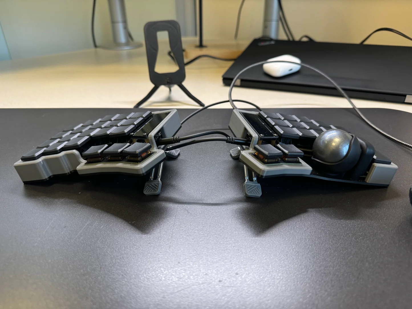
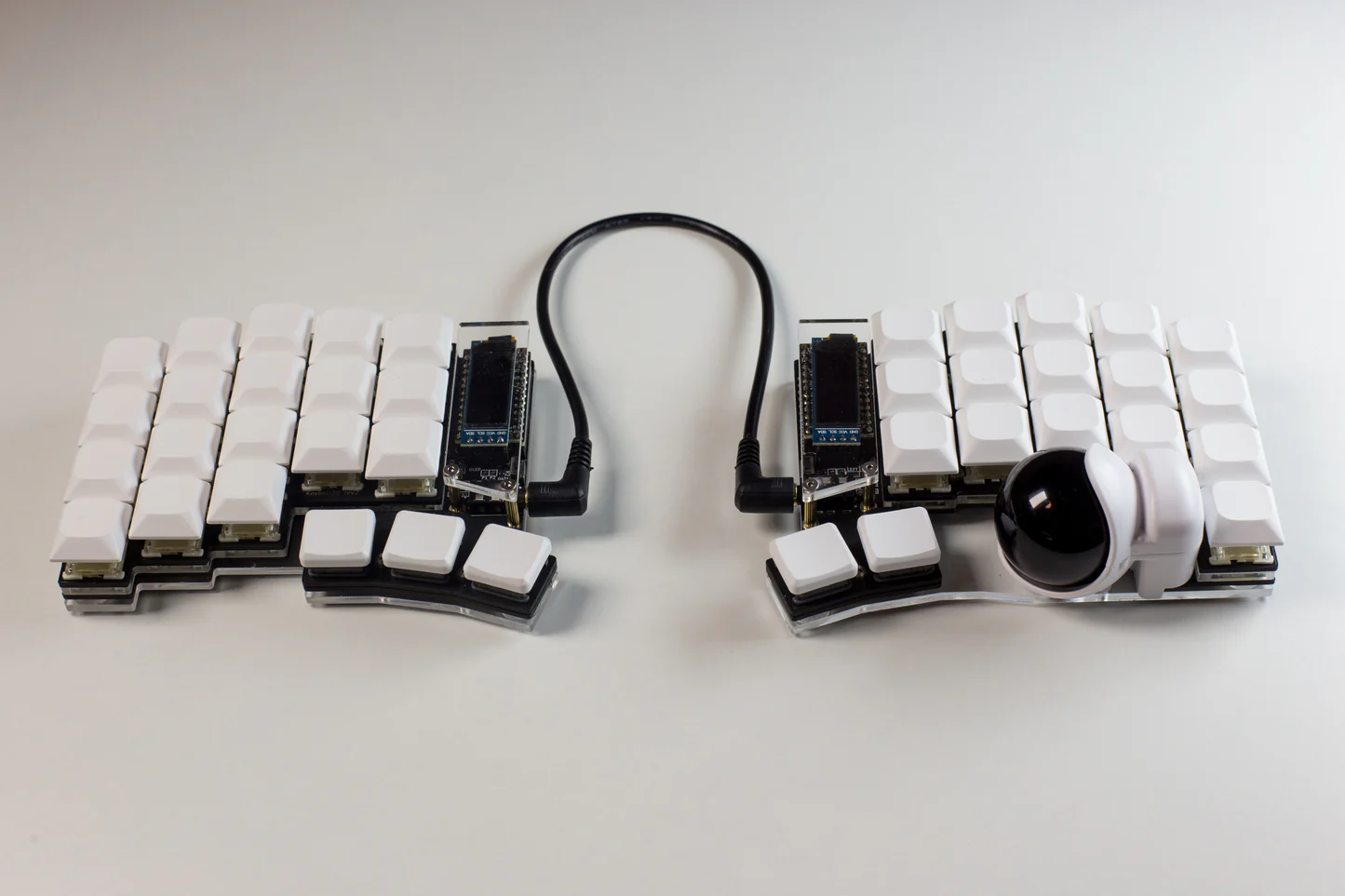
This article will discuss the keyball44, a 40% split keyboard design originally produced by Shirogane Labs.

This article will cover everything from where to purchase the keyboard, customization, and tips on how to adjust to a split keyboard.

Pros and Cons of a Split Keyboard

The Pros

Why a split keyboard? The main reason is ergonomics. You can position the halves of the keyboard such that your shoulders are in their natural position.

This is in contrast to a traditional keyboard where you can often find yourself in a hunched position. This is especially true if you’re a larger person.

Most split keyboards support tenting.

A tenting kit angles the keyboard halves upwards. This can help reduce wrist strain. The keyball44 includes an option for adding tenting legs.

The keyball44 is also a 40% keyboard. This means it has a smaller layout than traditional keyboards. This can be a pro or a con depending on your needs. On the pro side, the smaller layout means keys are easier to reach. Your hands barely move if at all.

Another pro of many split keyboards is their programmability. You can “flash” the keyboard with custom firmware. Through a flash, you can remap keys and create macros. The keyball44 supports QMK firmware. This means you can program the keyboard to your liking. You’ll see an example of one such mapping later on.

One pro of the keyball44 in particular is the trackball.

The trackball isn’t a one for one replacement for a mouse. That said, the trackball is accurate enough for most tasks and makes scrolling through long documents a breeze. It’s convenient to use a thumb on a trackball versus moving your hand to the mouse.

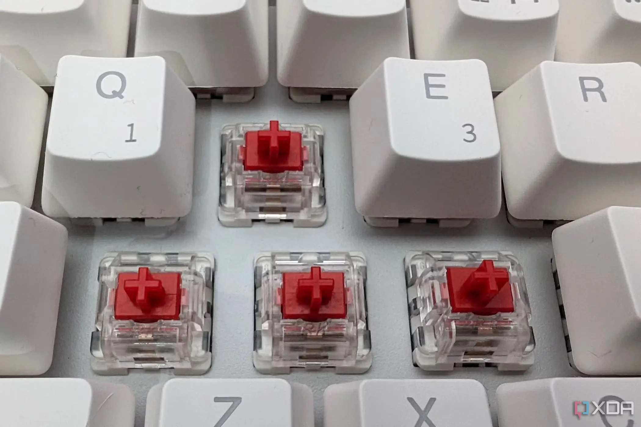
If you’re already a mechanical keyboard enthusiast, the keyball44 won’t disappoint. Most split keyboards support mechanical switches.

This means you can customize the feel of the keyboard to your liking. If you’re wondering what a switch is and why you should care, checkout this article for an in depth explanation.

Likewise, keycaps are often interchangeable. Keycaps not only change the look of the keyboard but they also can change the feel significantly.

The Cons

The main con of a split keyboard is the learning curve. If you’re used to a traditional keyboard, it can be difficult to adjust to a split keyboard. You’ll have to invest time into learning the new layout. The adjustment period can take anywhere from 2 weeks to a few months. How fast you adjust depends on how much you use the keyboard and how many sessions of deliberate practice you perform. 30 minutes a day of practice on a typing tutor site will get you back up to your original typing speed in no time. Here are some typing tutor sites you can try:

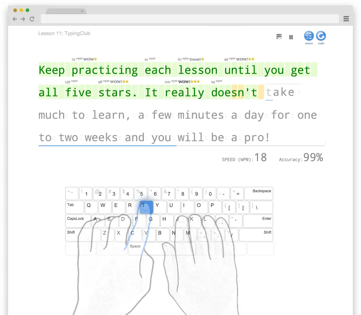
• TypingClub
• MonkeyType
• Keybr

TypingClub is the preferred option since it assumes no prior typing knowledge. TypingClub provides a structured approach that will have you practicing with most symbols and letters. If you’re new to touch typing, TypingClub is a great place to start.

Another con is the price. Split keyboards are often more expensive than traditional keyboards. And not just a little more expensive. The keyball44 starts at about $250. This is a lot of money for a keyboard. But if you’re serious about your health and productivity, it’s worth the investment.

How to Buy

It may seem silly to explain how to buy a keyboard, but the keyball44, much like other niche hardware, isn’t always easy to buy. There are a few options.

If you own a soughtering iron and you’re confident in your soughtering skills, you can build the keyboard yourself. There’s an official build guide that details everything you need to know. The guide includes a bill of materials and step by step instructions. To simplify the process even further, you can purchase build kits from various vendors. For example, HolyKeebs sells build kits that include (almost) everything you need.

Suck at soughtering? No problem. You can purchase a pre-built keyball44. For example, HolyKeebs sells pre-built keyball44s. HolyKeebs in particular provides various customization options including colors, keycaps, switches, and more. Not to mention they also sell additional equipment such as tenting kits and the TRRS cable required to connect the two halves of the keyboard. A keyball44 from HolyKeebs with modest customization and assembly will run you about 350 USD shipping included. Included in that price is about 75 dollars worth of assembly. If you purchase the tenting kit, cable, and trackball, you’ll be looking at about $400 all in.

One thing to keep in mind is that if you’re purchasing a pre-built board, you shouldn’t expect same day delivery. The lead time is usually about a month. Keep in mind that these aren’t mass produced. They’re made in small batches or even upon order by a small team of people.

Keymaps

The keyball44 supports QMK firmware. This means you can program the keyboard to your liking.

Since you’re working with the keyball44 which is a 40% keyboard and you’re new to split keyboards, you should start with a keymap optimized for 40% boards. “The Art of Making 40% Keyboards that Aren’t Crap” provides a solid starting keymap. The only modification required is the addition of a fifth layer for the trackball.

You can find a QMK ready keyball44 keymap that implements the fifth layer plus a few other tweaks here. Those tweaks include:

• Easier access to the mouse left and right button.
• A shortcut for shift+insert on the navigation layer.
• The arrow keys on the navigation layer are in a Vim style hjkl pattern.

If you want to further customize, you can find a keycode reference on the QMK site. If using a keyball44, you have access to additional keycodes. Check out the added keyball44 codes at HolyKeebs.

Flashing

Flashing the keyball44 is mostly straightforward. This article assumes you have a Linux PC running Arch Linux and a Windows PC.

Warning, when following the steps below, avoid connecting / disconnecting the TRRS cable when powered. This can short the GPIO pins of the controllers.

Follow these steps to flash the custom keymap introduced in Keymaps:

1. Clone the ieg-keyball44 branch of the QMK firmware repository fork:

git clone --branch ieg-keyball44 git@github.com:ivan-guerra/qmk_firmware.github
cd qmk_firmware

2. Install qmk:

sudo pacman -S qmk

3. Compile the keymap using qmk. Replace USER_NAME with your name. If your keyball44 doesn’t have a OLED screen, remove the -e OLED=yes option. If you have a board with RGB, add -e RGB=yes:

qmk compile -e USER_NAME=ieg -e OLED=yes -kb keyball/keyball44 -km ivan-guerra

4. Upon a successful build, you should see a keyball_keyball44_ivan-guerra.uf2 file in the top-level directory.

Size before:
   text	   data	    bss	    dec	    hex	filename
      0	  55372	      0	  55372	   d84c	keyball_keyball44_ivan-guerra.uf2

Copying keyball_keyball44_ivan-guerra.uf2 to qmk_firmware folder          [OK]

Transfer the file to your Windows PC.

5. Plug in the keyball44 to your Windows PC. Place the keyboard in bootloader mode by pressing the layer 5 modifier followed by the QK_BOOT key. See the default keymap for help locating those keys.

6. The keyboard will show up as a USB drive. Copy the keyball_keyball44_ivan-guerra.uf2 file to the USB drive.

7. Repeat the flash process this time plugging in the USB cable into the opposite half of the keyboard.

Conclusion

The keyball44 offers a compelling option for anyone looking to improve their typing comfort and ergonomics. This 40% split keyboard provides significant benefits including reduced shoulder strain, programmable layouts, and the convenience of an integrated trackball. While the learning curve and price present initial hurdles, the long-term health benefits and increased productivity justify the investment.

Start with a keymap that suits your workflow, practice consistently with typing tutors, and within a few weeks, you’ll likely find yourself typing comfortably and efficiently. The ability to fully customize both the hardware and firmware means your keyboard can evolve alongside your needs and preferences.

If you’re familiar with the demo-scene, you’ve probably seen the plasma effect:

In this article, you’ll learn how to implement plasma effects of your own.

The Algorithm

To generate a plasma effect, you iterate the pixels in the screen buffer. For each pixel:

1. Apply a function to the pixel’s coordinate producing some value $v$.
2. Use $v$ to calculate the new RGB value of the pixel.
3. Update the pixel’s RGB value in the screen buffer.
4. Repeat steps (1)-(3) until you have processed the entire image frame.
5. Display the updated frame.

Applying these steps at a high frequency creates the plasma animation. As you’ll see, the choice of function determines the shape and scale of the output image.

Plasma Functions

What function should you use when generating plasma? The sine function is popular due to its periodic nature. A vanilla sine function produces an image like the one shown below.

The white areas represent the peaks of the sine function, while the black areas represent the troughs. To produce more interesting plasmas, you can play with the function and its parameters.

The following sections describe a few functions you can use. In the equations that follow:

• $d$ is the distance from the center of the screen.
• $t$ is the time.
• $s$ is the scale factor.
• $\theta$ is the angle from the center point.
• $p_x$ and $p_y$ are the pixel’s coordinates relative to the center point.
• $d_{\min}$ is half of the smallest screen dimension.

Ripple

To produce a ripple effect, you can use the following function:

$$f(d, t, s) = \sin(ds - 2t)$$

Spiral

To produce a spiral effect, you can use the following function:

$$f(d, t, s, \theta) = \sin(ds + 3\theta + t)$$

Circle

To produce a circle effect, you can use the following function:

$$f(d, t, s, \theta) = \sin(ds + t) + \sin(2\theta + t)$$

Checkerboard

To produce a checkerboard effect, you can use the following function:

$$f(d, t, s, p_x, p_y, d_{\min}) = \sin\left(\frac{s p_x}{d_{\min}}\right) \sin\left(\frac{s p_y}{d_{\min}} + t\right)$$

Adding Some Color

In “The Algorithm” section, it’s mentioned you should use the value returned by the plasma function to calculate a pixel’s RGB color. How exactly do you do that? One way is to call a hsv_to_rgb() function. The hue argument to the hsv_to_rgb() varies as a function of the value returned by the plasma function:

let v = match self.shape {
    Shape::Ripple => self.ripple(dist, time),
    Shape::Spiral => self.spiral(dist, time, angle),
    Shape::Circle => self.circle(dist, time, angle),
    Shape::Square => self.square(px, py, min_dim, time),
};
// Normalize the plasma value from [-1,1] to [0,1] range for color mapping
let v = v * 0.5 + 0.5;

let (r, g, b) = match self.palette {
    Palette::Rainbow => self.hsv_to_rgb(v * 360.0, 1.0, 1.0),
    Palette::BlueCyan => self.hsv_to_rgb(v * 120.0 + 180.0, 0.8, 1.0),
    Palette::Hot => self.hsv_to_rgb(v * 60.0, 1.0, 1.0),
    Palette::PurplePink => self.hsv_to_rgb(v * 60.0 + 270.0, 0.7, 1.0),
}
*pixel = alpha | ((r as u32) << 16) | ((g as u32) << 8) | (b as u32);

The critical bit in the code is the hue value calculation. Hue is circular. The hsv_to_rgb() function expects the hue to be in the range ([0, 360]). The code maps the plasma value to the hue range of the desired palette. For example, a rainbow palette covers the full range of hues. In contrast, the blue/cyan palette covers 180–300 degrees of the hue circle.

Here’s a short clip showing the different plasma functions with various palettes:

Conclusion

Plasma effects demonstrate how simple mathematical functions can create mesmerizing animations. By combining sine waves, distance calculations, and color transformations, you can produce a variety of classic demo scene effects.

The complete project source is available on GitHub under plasma.

Port scanning is the name given to the process of discovering open ports on a remote host. In this article, you’ll explore the design and implementation of a basic port scanner written in Rust.

Starting with a Ping

Utilities with port scanning capabilities often start by sending a ping to the target. For example, nmap pings the target before scanning. This ensures the target is reachable.

To send a ping or an ICMP packet, you need to create a raw socket which requires the CAP_NET_RAW capability. A regular user doesn’t have CAP_NET_RAW capability meaning a ping requires sudo or elevated privileges. Luckily, modern Linux provides unpriviledged ping. The unpriviledged ping uses a dgram socket rather than a raw socket.

In Rust, the ping-rs crate provides an interface for sending pings using the unpriviledged method:

fn ping_host(addr: &IpAddr) -> PingApiOutput {
    let data = [0; 4];
    let timeout = Duration::from_secs(1);
    let options = ping_rs::PingOptions {
        ttl: 128,
        dont_fragment: true,
    };
    ping_rs::send_ping(addr, timeout, &data, Some(&options))
}

fn main() {
    match ping_host(&addr) {
        Ok(reply) => println!("Host is up ({}ms latency).", reply.rtt),
        Err(e) => return Err(format!("Host is unreachable, {:?}", e).into()),
    }
}

With these few lines of code, you’re able to check for connectivity. With connectivity established, you can proceed with port scanning.

Port Scanning Techniques

There’s a number of different approaches to port scanning. Which technique you select depends on the protocol you’re targeting and the level of stealth you want to maintain:

• TCP Connect Scan: This is the most common type of port scan. It involves attempting to establish a full TCP connection with the target port. If you successfully establish the connection, the port is open. If the target refuses the connection, the port’s closed.
• TCP Half Connect: This is a stealthier version of the TCP Connect Scan. It involves sending a SYN packet to the target port. If the port is open, the target will respond with a SYN-ACK packet. If the port’s closed, the target will respond with a RST packet.
• UDP Connect: This involves sending a UDP packet to the target port. If the target replies with any data, the port’s open. If the target responds with an ICMP port unreachable message, the port’s closed.

This article’s port scanner uses the TCP and UDP Connect techniques. Lets examine each technique and its code. Note, error handling isn’t shown in the snippets below. You can find the full source here.

Lets start with the TCP Connect Scan:

/// Attempts to establish a TCP connection to the specified address and determines the port state.
fn check_tcp_connection<A: ToSocketAddrs>(addr: A, timeout_ms: u64) -> Option<PortState> {
    let target = addr
        .to_socket_addrs()
        .expect("Error getting socket addrs")
        .next()
        .unwrap();

    match TcpStream::connect_timeout(&target, Duration::from_millis(timeout_ms)) {
        Ok(_) => Some(PortState::Open),
        Err(e) if e.kind() == std::io::ErrorKind::ConnectionRefused => Some(PortState::Closed),
        Err(_) => Some(PortState::Filtered),
    }
}

check_tcp_connection() attempts to establish a TCP connection to the target. If it opens the connection, the port is open. If the target refuses the connection, the port’s closed. Otherwise, you can assume a firewall or some other network filter is filtering the port. The timeout controls the duration of the connection attempt. You don’t want to attempt to connect and block forever, hence the timeout. That said, how long should you block? Since you may scan up to 65535 ports, you don’t want the timeout to be too large else the scan will take too long. Make the timeout too short and you may miss out on open ports. This parameter should be tunable by the user so that they can decide how aggressively they want to scan.

Here’s the UDP Connect Scan:

/// Checks the state of a UDP port by sending an empty datagram and analyzing the response.
fn check_udp_port(socket: &UdpSocket, addr: &str) -> Option<PortState> {
    let target_addr = addr
        .to_socket_addrs()
        .expect("Failed to resolve address")
        .next()
        .unwrap();

    socket
        .send_to(&[], target_addr)
        .expect("Failed to send UDP packet");

    let mut buffer = [0u8; 512];
    loop {
        match socket.recv_from(&mut buffer) {
            Ok((_, src_addr)) => {
                // If we receive any data, consider the port Open
                if src_addr.to_string() == addr {
                    return Some(PortState::Open);
                }
            }
            Err(ref e) if e.kind() == io::ErrorKind::WouldBlock => {
                // Timeout reached, port is considered Filtered
                return Some(PortState::Filtered);
            }
            Err(ref e) if e.kind() == io::ErrorKind::ConnectionReset => {
                // ICMP Destination Unreachable received
                return Some(PortState::Closed);
            }
            Err(_) => return None, // Handle other unexpected errors
        }
    }
}

check_udp_port() is similar to check_tcp_connection(). The key difference is that since UDP is connectionless, you need to analyze the response to determine the port state. A reply from the target indicates the port is open. An ICMP port unreachable message indicates the port’s closed. If you don’t receive a reply, you can assume the port’s filtered by a firewall or some other network filter.

Scanning in Parallel

Scanning ports sequentially is slow. When using a connection timeout of 25 milliseconds for each port, scanning all 65535 ports could take up to 27 minutes. To speed up the scan, you can scan ports in parallel. The secret is to chunk the port range based on the number of cores available on the host.

Here’s the relevant snippet taken from the UDP scanner:

/// Performs a UDP port scan on the specified IP address within the given port range.
///
/// The scan is performed using multiple threads (up to 16) to improve performance.
fn scan(
    &self,
    addr: &std::net::IpAddr,
    port_range: &PortRange,
    timeout_ms: u64,
) -> ScanResults {
    let ports: Vec<u16> = (port_range.start..=port_range.end).collect();
    let n_threads = num_cpus::get().min(16);
    let chunk_size = ports.len().div_ceil(n_threads);
    let target = Arc::new(*addr);
    let results = Arc::new(Mutex::new(ScanResults::new()));

    let handles: Vec<_> = ports
        .chunks(chunk_size)
        .enumerate()
        .map(|(i, chunk)| {
            let addr = Arc::clone(&target);
            let results = Arc::clone(&results);
            let ports = chunk.to_vec();

            thread::Builder::new()
                .name(format!("udp-scanner-{}", i))
                .spawn(move || {
                    // Call check_udp_port()
                })
                .expect("Failed to spawn thread")
        })
        .collect();

    for handle in handles {
        if let Err(e) = handle.join() {
            eprintln!("Thread panicked: {:?}", e);
        }
    }

    let mut results = Arc::try_unwrap(results)
        .expect("Failed to unwrap Arc")
        .into_inner()
        .expect("Failed to acquire mutex lock");
    results.sort_by(|a, b| a.port.cmp(&b.port));

    results
}

Here are the highlights. n_threads uses the num_cpus crate to determine the number of logical cores on the host. The value gets clamped down to a maximum of 16. chunk_size calculates the number of ports each thread will scan. handles is a vector of thread handles. Each handle represents a thread that will scan a chunk of ports. The program joins all threads and sorts the results by port number for display.

The speed up achieved by this code is significant. Many cases saw an upwards of 50% reduction in scan time versus a sequential scan.

Displaying Service Names

One handy feature many port scanners support is the ability to display the service name associated with a port. For example, one might see the service name “https” associated with port 80.

The Internet Assigned Numbers Authority (IANA) maintains a list of well-known port numbers and the services associated with them. You can visit the IANA website and browse the port to service mappings.

When printing port numbers and statuses, it’s a good idea to include the service name:

PORT       STATE      SERVICE
22/udp     filtered   ssh
23/udp     filtered   telnet
24/udp     filtered   unknown
25/udp     filtered   smtp
26/udp     filtered   unknown
27/udp     filtered   nsw-fe
28/udp     filtered   unknown
29/udp     filtered   msg-icp

Hostname Resolution

Another useful scanner feature is the ability to resolve hostnames. A user might not want to enter a raw Ipv4/IPv6 address. Instead, they might want to enter a hostname such as gnu.org or reddit.com. Hostname resolution is straightforward in Rust:

/// Resolves a hostname to its corresponding IP address.
pub fn resolve_hostname_to_ip(hostname: &str) -> Option<IpAddr> {
    let addr = format!("{}:0", hostname);
    addr.to_socket_addrs()
        .ok()
        .and_then(|mut iter| iter.next()) // Take the first resolved address
        .map(|socket_addr| socket_addr.ip())
}

The to_socket_addrs() function returns a iterator over the resolved addresses. The code takes the first address and returns it. Simple as that.

Conclusion

Port scanning is a useful tool for network administrators and hackers alike. In this article, you’ve seen how to implement a basic port scanner in Rust. The scanner supports both TCP and UDP scanning techniques. It scans ports in parallel to speed up the process. It displays the service name associated with each port and resolves hostnames to IP addresses. There’s plenty of other features you could add to this scanner. If you’re further interested, checkout “real-world” scanners like NetCat, Angry IP Scanner, and nmap.

pscan implements the ideas discussed in this article. The complete project source is available on GitHub under pscan.

A previous article explored writing rsbot, a scriptable auto clicker meant to automate training the most repetitive skills in RuneScape. As a recap, that bot would take as input a script defining click events where each click event includes an ID, click box, and delay range. The bot would continuously execute each event. Executing an event means randomly clicking within the click box and waiting a random amount of time within the delay range. Bonus points, rsbot mouse movements look human.

rsbot works well. It allowed a main account to level fletching, firemaking, herblore, crafting, and many other skills to 99 without catching even a temp ban. However, certain skills require more than just an “intelligent” auto clicker. For example, when training fishing, the fishing spot occasionally moves. Or when woodcutting, you want to know when the tree gets cut and immediately move to cutting another tree. The common thread amongst these skills is that the resources aren’t completely static. The bot needs to react to random in game events.

A desire to continue botting tedious skills motivates the development of colorbot. Much like rsbot, colorbot is scriptable meaning you can write scripts to bot whichever skill you like. The key difference is that instead of hard coding click boxes, colorbot uses color recognition to guide its clicks.

Color Recognition

The color recognition aspect of the bot is stupid simple. The process is:

1. Take a screenshot.
2. Find all pixels in that screenshot matching a target color.
3. Click one of those pixels at random.

That’s it. No fancy graph algorithms, probability, nothing. Of course, there are a couple gotchas with this approach.

First, you must specify a color tolerance. You might get the color of a pixel in game and then find that the bot can’t detect it because you moved the camera slightly. Shadow and lighting effects can change the color of a pixel. The solution is to specify a color and a tolerance. The tolerance applies to each RGB component of the pixel. The algorithm matches any pixel within tolerance.

Second, you may find that many objects on screen share the same color as your target leading to false positives. One solution is to make the colors of the objects distinctive. Most objects’ pixels have color components with mixed values. What you want is to have “unique” colors with respect to the common colors in the game. For example, red $(255,0,0)$, green $(0,255,0)$, and cyan $(0,255,255)$ don’t occur in RuneScape. You might ask, if they don’t occur, how can you use these colors as targets? You can leverage features of the game client to make a viable solution. This article provides examples of how to do this.

Performance

You want the color detection process to be quick. rsbot is a Python script. Screen capturing and iterating over all pixels in a $1920 \times 1080$ image is noticeably slow in Python. Rather than optimizing the Python code, it’s easier to translate the useful parts of rsbot to a compiled language. colorbot is a Rust application but any other compiled language such as C or C++ would work just as well.

A benefit of using Rust is its package manager, Cargo. With Cargo, it’s straightforward to install a cross platform screen capture library. colorbot uses the scrap crate to take screenshots. Below is the bulk of the color matching code:

/// Captures the screen and finds all pixels matching a target color within a tolerance
pub fn get_pixels_with_target_color(
    target_color: &(u8, u8, u8, u8),
) -> Result<Vec<Point>, Box<dyn std::error::Error>> {
    // Get the primary display
    let display = Display::primary()?;
    let width = display.width();
    let mut capturer = Capturer::new(display)?;
    let mut matches = Vec::new();
    const TOLERANCE: u8 = 10;

    loop {
        // Try to capture a frame
        if let Ok(frame) = capturer.frame() {
            // Iterate over the pixels
            for (i, pixel) in frame.chunks(4).enumerate() {
                // Pixels are in BGRA format
                let b = pixel[0];
                let g = pixel[1];
                let r = pixel[2];
                let a = pixel[3];

                if color_matches((b, g, r, a), *target_color, TOLERANCE) {
                    // Calculate pixel coordinates
                    let x = i % width;
                    let y = i / width;
                    matches.push(Point::new(x as f64, y as f64));
                }
            }

            break; // Exit after one frame
        }
    }

    Ok(matches)
}

The code iterates over the BGRA pixels in the screenshot and checks if each pixel matches the target color. After finding a match, the code stores the pixel’s coordinates in a vector. The function returns the vector of matching pixels. For an $M \times N$ image, this function has a time complexity of $\mathcal{O}(MN)$. Not winning any performance awards but it’s fast enough for this purpose.

Scripting

Scripting is one of the most important features of colorbot. The bot accepts a JSON file containing a list of click events. Each click event has a string ID, a list of color components, and a list representing the post-click delay range. Below is an example script for fishing:

{
  "events": [
    {
      "id": "lure fish",
      "color": [252, 23, 35],
      "delay_rng": [75000, 80000]
    },
    {
      "id": "drop fish 1",
      "color": [171, 32, 253],
      "delay_rng": [100, 200]
    },
    {
      "id": "drop fish 2",
      "color": [171, 32, 253],
      "delay_rng": [100, 200]
    },
    ...
  ]
}

The script demonstrates three events. The first, lure fish, clicks a fishing spot and waits between 75000 to 80000 milliseconds. The other events click to drop a fish in the inventory and wait between 100 to 200 milliseconds. The delay exists to accommodate certain long actions. The delay varies to avoid detection by Jagex’s bot detection system. Disclaimer, it’s unknown whether randomizing mouse gestures, delays, etc. actually helps but it’s better to be safe than sorry.

Leveraging Game Client Features

It would be disingenuous to say that colorbot is a completely standalone bot. For it to work, you need to use some plugin features of the game client. Specifically, the RuneLite game client.

The first critical plugin is the NPC Indicator plugin. NPC Indicator highlights NPCs on screen. You can customize the colors and the highlight styles. Here’s a short video from the developer’s demonstrating how it works:

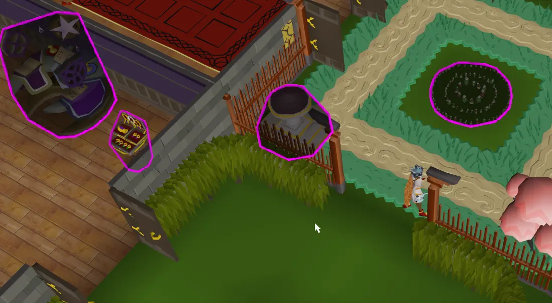
RuneScape has many surprising elements that register as NPCs. For example, fishing spots are all NPCs! Configure the plugin and your colorbot script to use colors which don’t occur in the game such as pure red, green, etc. This guarantees you’ll accurately click the object you’re interested in.

What if you want to click non NPC objects? You can mark arbitrary objects using the Object Markers plugin. You can customize the color and highlight style here as well:

Just shift click the object you want to mark and select the color and additional options from the pop-up menu.

Next up, coloring items in your inventory. For this, the Inventory Tags plugin is useful. Checkout this short clip demoing usage:

Finally, the Menu Entry Swapper plugin lets you avoid right clicking and searching through menus. This is useful in many ways. For example, say you want to drop an inventory of logs. You can set the left click option on logs to “drop.”

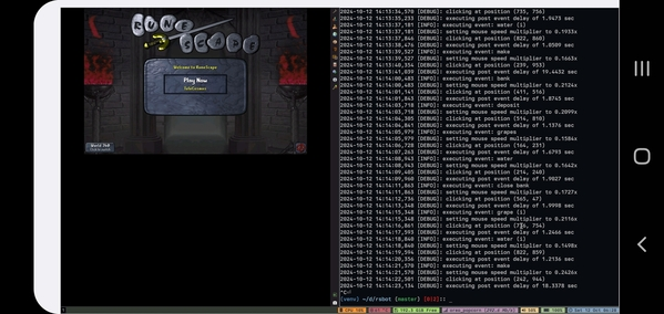
Configuring four plugins alongside colorbot might sound like a lot of work. However, you’ll find that spending 45 minutes to an hour configuring the bot is much less painless than manually skilling for 200 hours or more. Below is an example of a fishing script in action (note, the video is a bit slow since the PC was overloaded at the time of recording):

The NPC Indicator Plugin highlights the fishing spots red. The Inventory Tags Plugin highlights the fish in the inventory purple. colorbot runs a fishing script which uses the information on screen to click a luring spot and drop fish in the inventory. This script ran 12 hours a day for close to a month on the journey from 67 to 99 fishing. You can do the math on how many hours that saved.

Conclusion

colorbot demonstrates how color-based automation can be both simple and effective. While this approach has limitations, it works well for automating skills with random elements in RuneScape. Client plugins play a crucial role in this setup. Without plugins to highlight key elements with distinct colors, colorbot would be unable to reliably identify and interact with game objects.

The complete project source is available on GitHub under colorbot.

Update: colorbot nearly got a main account to max without a ban. Two skills remained before a temporary two day ban was issued for a macro minor offense. Agility and farming had to be leveled manually. The bot was banned 4 days into agility training. The bot ran for 12 hours a day in 3 hour sessions with 1.5 to 2 hour breaks between sessions. This worked fine for all previous skills. However, for agility, I started running 15 hours a day. I suspect this is what triggered the ban. Moral of the story, don’t run the bot excessively. I speculate that running the bot for 9 hours a day with metered breaks is the sweet spot. Despite the ban, I did suffer the last two skills to achieve my childhood goal of maxing on RuneScape.

This post includes the notes made while reading the article titled “C++ Design Patterns for Low-Latency Applications Including High-Frequency Trading” by Paul Bilokon and Burak Gunduz.

Section 2: Background

2.1 HFT

• High-frequency trading (HFT) is an automated trading strategy that utilises technology and algorithms to execute numerous trades at high speeds.
• The SEC Concept Release on Equity Market Structure outlines five key elements that define this discipline:
  • High-speed computing.
  • Co-location practices.
  • Short time frames for position establishment and liquidation.
  • The submission of multiple orders followed by cancelled orders.
  • The objective of concluding the trading day with minimal unhedged positions and near-neutral exposure to overnight.
• HFT systems are mainly built from five main components:
  • Data Feed: Responsible for receiving and processing real-time market data from various sources, enabling the algorithms to make buy, sell, or wait decisions.
  • Order Management System (OMS): Handles the submission, routing, and monitoring of trade orders, ensuring efficient execution and management of trading activities.
  • Trading Strategies: Employ automated algorithms to identify market opportunities, make trading decisions, and execute trades at high speeds.
  • Risk management: Implements measures to assess and mitigate potential risks associated with high-speed trading, ensuring the preservation of capital and minimizing losses.
  • Execution Infrastructure: Provides the necessary technological framework for low-latency communication and trade execution in HFT systems. Networking infrastructure falls in this category.
• HFT firms make strong use of Field Programmable Gate Arrays (FPGAs) to achieve low-latency targets. Four key characteristics of FPGAs are programmability, capacity, parallelism, and determinism.

2.2 C++

• HFT shops prefer C++ for low-latency applications due to its compiled nature, close proximity to hardware, and control over resources, which enables you to optimize performance and efficiently manage resources.
• C++ offers various techniques to shift processing tasks from runtime to compile-time. Examples include:
  • Using templates to move the runtime overhead associated with dynamic polymorphism to compile-time in exchange for flexibility.
  • Inline functions which insert a function’s code at the call site.
  • The constexpr keyword evaluates computations at compile time instead of runtime, resulting in quicker and more efficient code execution.
• Factors such as the compiler (and its version), machine architecture, 3rd party libraries, build and link flags can also affect latency.
• It’s often necessary to view the generated assembly when benchmarking C++. Tools such as Matt Godbolt’s Compiler Explorer help you do just that.

2.3 Design Patterns

Design patterns in this paper don’t refer to object oriented design patterns. Instead, the authors use the term “design patterns” to refer to a number of programming strategies. Here’s a list of the different programming strategies:

• Cache Warming: To minimize memory access time and boost program responsiveness, preload data into the CPU cache before it’s needed.
• Compile-time Dispatch: Through techniques like template specialization or function overloading, the compiler can choose optimised code paths at compile time based on type or value, avoiding runtime dispatch and early optimisation decisions.
• Constexpr: Computations marked as constexpr evaluate at compile time, enabling constant folding and efficient code execution by eliminating runtime calculations.
• Loop Unrolling: Loop statements expand during compilation to reduce loop control overhead and improve performance, especially for small loops with a known iteration count.
• Short-circuiting: Logical expressions cease evaluation after computing the final result, reducing unnecessary computations and improving performance.
• Signed vs Unsigned Comparisons: Ensuring consistent signedness in comparisons avoids conversion related performance issues and maintains efficient code execution.
• Avoid Mixing Float and Doubles: Consistent use of float or double types in calculations prevents implicit type conversions, potential loss of precision, and slower execution.
• Branch Prediction/Reduction: Accurate prediction of conditional branch outcomes enables speculative code execution, reducing branch misprediction penalties and improving performance.
• Slowpath Removal: Optimisation technique aiming to minimize execution of rarely executed code paths, enhancing overall performance.
• SIMD: Single Instruction, Multiple Data (SIMD) enables a single instruction to operate on multiple data points simultaneously, significantly accelerating vector and matrix computations.
• Prefetching: Explicitly loading data into cache before it’s needed can help in reducing data fetch delays, particularly in memory-bound applications.

2.4 LMAX Disruptor

• The LMAX Disruptor addresses the specific requirements of their high performance, low-latency trading system.
• The LMAX Disruptor offers a highly optimised and efficient messaging framework that enables concurrent communication between producers and consumers with minimal contention and latency.
• The LMAX Disruptor addresses the issue of shared resource contention between multiple threads. The cost comes from context switches. Those context switches can invalidate the cache or even lead to a cache flush which hurts performance. When the new thread starts, the cache for that task likely needs to build up which incurs some additional latency.
• Another way to tackle contention is the use of Compare And Swap (CAS) operations. CAS is an atomic instruction used in concurrent programming to implement synchronization and guarantee data integrity in multi-threaded environments.
• You can implement lock-free data structures using CAS instructions.
• Using CAS instructions directly comes at a cost:
  • Orchestrating a complex system using CAS operations can be harder than the use of locks.
  • To guarantee atomicity, the processor locks its instruction pipeline, and a memory barrier ensures that changes made by a thread become visible to other threads.
• Producer/consumer queues are common in HFT code. Unbounded queues are problematic due to the possibility of memory exhaustion caused by producers outpacing consumers. Bounded queues solve the memory issue at the cost of increased write contention on the head, tail, and size variables. This can be made worse by cache coherency issues.
• The LMAX Disruptor uses a preallocated ring buffer. In most use cases, there is one producer (for example, a file reader or network listener) and multiple consumers. A single producer means there’s no contention on entry allocation. Producers notify waiting consumers when data is available. Many read-only consumers can safely access the data simultaneously. Notice, how the LMAX Disruptor strategy avoids CAS contention present in other multi-producer multi-consumer queues.
• Producers and consumers interact with the ring buffer based on sequencing. Producers claim the next available slot in the sequence. Once the producer claims a slot, the producer can write to it and update a cursor representing the latest entry available to consumers. Consumers wait for a specific sequence by using memory barriers to read the cursor, ensuring visibility of changes. Consumers maintain their own sequence to track their progress and coordinate work on entries.
• The Disruptor offers an advantage over queues when consumers wait for an advancing cursor in the ring buffer. If a consumer notices that the cursor has advanced multiple steps since it last checked, it can process entries up to that sequence without involving concurrency mechanisms. This enables the consumer to catch up with producers during bursts, balancing the system. This batching approach improves throughput, reduces latency, and provides consistent latency regardless of load until the memory system becomes saturated.

2.5 Benchmarking

• Google Benchmark is a benchmarking library offering support for CPU-bound and real-time modes. The library performs multiple iterations of specific code snippets or functions, thereby generating accurate performance metrics.
• Google Benchmark might not cover some specifics unique to HFT scenarios, such as network latency, co-location effects, and hardware timestamping, among others. You must supplement with other performance analysis tools that can analyze these additional factors.
• Performance Counter for Linux or perf is a sophisticated performance monitoring utility that integrates into the Linux kernel. It provides a rich set of commands and options for profiling and tracing software performance and system events at multiple layers, from hardware-level instruction cycles to application-level function calls.
• The authors of this paper used perf for cache analysis.

2.6 Cache Analysis

• The ratio of cache hits to total access attempts is often used as an important metric for evaluating the effectiveness of a cache system.

2.7 Networking

• Low-latency networks are the linchpin of high-frequency trading. The propagation delays in transmitting information can have immediate financial implications.
• Most HFT firms opt for fiber-optic communication to enable data transmission at speeds close to the speed of light.
• Colocation remains a crucial strategy for HFT firms, providing them the benefit of proximity to a stock exchange’s data center, thus further minimizing latency.
• Another critical aspect is the network topology used within the trading infrastructure. The design of these networks focuses on maximizing speed and minimizing the number of hops between network nodes. This often involves direct connections between key components in the trading infrastructure, thereby avoiding potential points of latency and failure.
• Redundancy measures are usually put in place, including dual network paths, failover systems, and backup data centers to maintain a 100% uptime.
• Additionally time is a critical factor in high-frequency trading, and the use of precise time-synchronization protocols like Precision Time Protocol (PTP) is becoming increasingly important. Accurate timestamping of events enables for fairer market conditions and is often a regulatory requirement.

Section 3: Low-Latency Programming Repository

The Low-Latency Programming Repository divides into five categories: compile-time features, optimization techniques, data handling, concurrency, and system programming.

3.1 Compile-Time Features

• In HFT, the execution path that reacts to a trade signal is the hot path.
• Cache warming pre-loads the necessary data and instructions for the hot path into the cache. The hotpath is typically kept warm by executing the hot path code frequently. Orders are actually only released when a trade executes.
• Runtime dispatch and compile-time dispatch are two techniques in object-oriented programming that determine which specific function gets executed.
• Runtime dispatch, also known as dynamic dispatch, resolves function calls at runtime.
• Compile-time dispatch determines the function call during the compilation phase and is frequently used in conjunction with templates and function overloading.
• The benefit of compile-time dispatch stems from the ability of the compiler to inline the functions that would have been virtual. Inlining can unlock further optimizations. See “The cost of dynamic (virtual calls) vs. static (CRTP) dispatch in C++” for more info.
• Sources of the runtime cost of virtual calls:
  • Extra indirection (pointer dereference) for each call to a virtual method.
  • Virtual methods usually can’t be inlined, which may be a significant cost hit for some small methods.
  • Additional pointer per object. On 64-bit systems which are prevalent these days, this is 8 bytes per object. For small objects that carry little data this may be a serious overhead.
• Constexpr is a keyword in C++ facilitating the evaluation of expressions during compilation rather than runtime.
• The primary objective of the constexpr keyword is to shift computations from runtime to compile-time, not necessarily to boost runtime velocity.
• Inlining refers to a compiler optimisation method in which a function call is replaced by the actual content of the function. This procedure aims to reduce the overhead typically linked with function calls, such as parameter transmission, stack frame handling, and the function call return process.

3.2 Optimization Techniques

• Loop unrolling is a technique used in computer programming to optimise the execution of loops by reducing or eliminating the overhead associated with loop control. It’s a form of trade-off between processing speed and program size.
• Short-circuiting is a logical operation in programming where the evaluation of boolean expressions stops as soon as you have the final result. Short-circuiting consistently results in faster execution. Short-circuit where possible.
• Separating slowpath code from the hotpath can significantly enhance latency in code execution. The strategy is encapsulate the slow path operations (for example, error handling) so as to keep the hotpath lean. The end result is that the instruction cache gets used more efficiently leading to a reduction in execution time. It’s recommended to not inline the slow path functionality so as to not unintentionally bloat the icache.
• By minimising unnecessary branches and avoiding potential branch mispredictions, you can reduce program latency significantly.
• Prefetching is a technique used by computer processors to boost execution performance by fetching data and instructions from the main memory to the cache before it’s actually needed for execution. Functions like __builtin_prefetch can assist in the prefetching of data.

3.3 Data Handling

• Unsigned comparisons take longer than signed comparisons. This caused by the fact the compiler must insert instructions to check for wrap around on the unsigned value. This can be costly when loop control uses unsigned values.
• Mixing data types specifically float and double can introduce additional latency. float types are automatically promoted to double when in a computation with at least one double type. According to the article, the conversion to and from float can cause an up to 50% slow down compared to using float directly.

3.4 Concurrency

• SIMD, or Single Instruction Multiple Data, is a category of parallel computing architectures where a single instruction can act upon multiple data points simultaneously.
• The SIMD architecture’s capability to process multiple data points concurrently leads to increased data throughput and reduced latency, features especially beneficial for operations involving large data sets or arrays.
• Lock-free programming is a concurrent programming paradigm that centers around the construction of multi-threaded algorithms which don’t employ the usage of mutual exclusion mechanisms, such as locks, to arbitrate access to shared resources.
• The process of locking can be computationally expensive, necessitating system calls and occasionally leading to the suspension of the calling thread if the lock is presently held by an alternate thread. In contrast, atomic operations are typically implemented using CPU instructions and don’t demand context switches, thus conferring upon them a superior speed profile.
• Performance improvements gained through lock-free programming may vary based on numerous factors, including hardware specifications, number of threads, and the workload’s contention level.

Closing Remarks

The rest of the article goes on to show the design patterns applied to a statistical arbitrage pairs trading strategy. The authors also implement a queue following the LMAX disruptor pattern. They conclude with data showing how the combination of the design patterns and LMAX disruptor produce a significant reduction in their strategies’ latency compared to a naive/unoptimized approach.

Perhaps the design patterns described by the authors aren’t particularly ground breaking. That said, their “Low Latency Programming Repository” is unique. Having not only the descriptions of the design patterns in the article, but a repository with clear examples is the true highlight.

Have you been away from your PC and wished you could login and start a job or view a file? Do you run Linux on your PC and use an Android phone? If you answered yes to these questions, you came to the right place. In this article, you’ll see how to connect to and control your Linux PC from anywhere in the world using your Android phone.

Required Software

On your Linux PC, install the following packages using your distro’s package manager:

• TigerVNC
• OpenSSH

On your Android device, install the following apps via the Google PlayStore:

• ConnectBot
• androidVNC

PC Side Setup

On the PC side, you need to standup the VNC server and the OpenSSH service.

VNC Server

The “TigerVNC on Linux” article goes into detail on setting up a TigerVNC client/server on Linux. In this case, you only need to configure and launch the TigerVNC server. Follow the steps below to setup the server on your Linux PC:

1. Create a password by running vncpasswd. The password file saves to $XDG_CONFIG_HOME/tigervnc/passwd. Make sure passwd has its permissions set to 0600.

2. Add users by editing /etc/tigervnc/vncserver.users. Below is an example vncserver.users file containing a single user, ieg, assigned to display :1:

:1=ieg

3. Create $XDG_CONFIG_HOME/tigervnc/config. Below is an example configuration. Set session and geometry according to your needs. Note, session is the name of the desktop environment installed on your PC. You can run echo $XDG_CURRENT_DESKTOP to retrieve the desktop name.

session=i3
geometry=1920x1080
localhost
alwaysshared

4. Start your VNC server service using systemd. Set the display number to match the display number you configured in vncserver.users. For example:

sudo systemctl start vncserver@:1.service

OpenSSH

1. Edit /etc/ssh/sshd_config (requires sudo) and set the GatewayPorts setting to yes.
2. start/enable the sshd service:

sudo systemctl start sshd

To add a bit of security to your SSH config, apply these settings to sshd_config:

• Specify what users may SSH to the PC by defining AllowUsers. For example, AllowUsers foo bar makes it so only the users foo and bar can SSH to the PC.
• Disallow root login by setting PermitRootLogin no.
• Change the SSH port from the default $22$ to some random, unused port. You can set the option using the Port config item. For example, Port 31456. Valid ports are in the range $[1024, 65535]$. Just be sure to pick a port that isn’t used by some other application.
• Set PasswordAuthentication no. This makes it so you can only enable login via public key authentication.

After saving your settings, restart the sshd service:

sudo systemctl restart sshd

Router Setup

You will need to configure port forwarding on your home router to enable SSH traffic into your home network. If you have you’re own router, you can login into the router and setup the rule. If you rent a router from an ISP, most ISPs provide an app that includes an “Advanced Settings” section from which you can setup port forwarding rules. Download the app and create the rule.

Below is an example of how you would setup SSH port forwarding using an Xfinity provided router:

1. Sign in to the Xfinity app with your Xfinity ID and password.
2. Select “WiFi” from the bottom navigation.
3. Select “View WiFi” equipment.
4. Select “Advanced Settings.”
5. Select “Port forwarding.”
6. Select “Add Port Forward” and continue to the next screen.
7. Select the home equipment to redirect ports from the menu of connected devices.
8. Setup the forwarding rule. If you followed the advice at the end of OpenSSH and changed the SSH port from the default $22$, then enter the port number you set in sshd_config.

Here’s an example Xfinity port forwarding rule for SSH:

prim is the name of the Linux PC on the LAN. $54446$ is the port configured for SSH on the PC. It’s fine to leave the protocol set to the “TCP/UDP” option.

Android Device Setup

On the Android device, you only need to configure settings within the ConnectBot and androidVNC applications.

ConnectBot

1. Open the ConnectBot app, and tap the ”+” symbol at the bottom right to add a new host.
2. Fill in the details in the “username@hostname:port” field. Username is the username of a whitelisted SSH user on the Linux PC. Hostname is the IPv4 address of your PC. You can find this information by logging into the PC and going to whatismyip.com. Port is the SSH port. The default value is $22$. If you followed the security advice at the end of OpenSSH, then be sure to set the port to match the Port setting in your PC’s sshd_config.
3. Tap “Use pubkey authentication” and select the “Use any unlocked key” option.
4. Save your settings and return to the ConnectBot home screen.
5. Select the vertical ellipses at the top right of the screen and tap on “Manage Pubkeys.”
6. Add a new key by tapping ”+” at the top right of the screen. The default 2048 bit RSA key settings are fine. Tap “Generate Key” when you’re done making your selections and follow the prompts to generate entropy.
7. In the Pubkeys page, unlock your key by tapping it until the icon changes to that of an unlocked lock. Press and hold your key in the drop down and select “Copy public key.”
8. Transfer the public key to your Linux PC via email or some other means. On your Linux PC, add the public key to the SSH users’ ~/.ssh/authorized_users file.
9. Back on the Android device, verify you can login to your PC via ConnectBot. Tap your host on the hosts page. You should see a shell like the one shown below.
10. From within the shell session, tap the vertical ellipses in the top right corner and select “Port Forwards.”
11. Add a new port forwarding rule with type set to “Local,” source port set to $5901$ and destination set to “127.0.0.1:5901.”

androidVNC

1. Open the androidVNC app. You should be immediately prompted to create a new connection.
2. Fill out the following fields. Set “Nickname” to whatever you would like to call this connection. “Password” is the VNC password you set on the server. “Address” is $127.0.0.1$. “Port” is $5901$. All other settings can be left at their defaults.
3. Tap “Connect” in the top left to connect to your VNC server.
4. You should see your PC desktop loading. The first frame may take awhile to load.

After following the steps, did you get the following error message?

Verify in the ConnectBot app your SSH connection to the Linux PC is active. The SSH connection must be active with the port forwarding rule enabled, else the androidVNC connection won’t make its way through to the server.

Virtual Network Computing or VNC makes it possible to remotely access the graphical desktop environment of another machine. There are a number of projects out there that implement the VNC protocol. Typically, these projects provide two applications: a VNC server and a VNC client. The remote target machine runs the VNC server program. A VNC client instance connects to the target’s VNC server. The client application is a GUI application that renders the graphical display of the remote target. The image below illustrates the concept:

In this article, you’ll see how to setup a VNC server and client on Linux using TigerVNC.

Prerequisites and Assumptions

This article assumes you are on an Arch Linux machine with an Internet connection. That said, the instructions that follow should work for any Linux distro though the package installation commands will certainly need tweaking.

Step-By-Step

TigerVNC is the recommended VNC implementation. TigerVNC provides both the client and server application. To install TigerVNC, run the following command:

pacman -S tigervnc

VNC Server Setup

1. Create a password by running vncpasswd. The password file saves to $XDG_CONFIG_HOME/tigervnc/passwd. Make sure passwd has its permissions set to 0600.

2. Add users by editing /etc/tigervnc/vncserver.users. User entries consist of both a display number and username. You can spawn multiple server instances, one per display. Note, the display number is automatically associated with a TCP port. For example, display :1 binds to port $5900 + 1 = 5901$, display :2 binds to port $5900 + 2 = 5902$, etc. Below is an example vncserver.users file containing a single user:

# TigerVNC User assignment
#
# This file assigns users to specific VNC display numbers.
# The syntax is <display>=<username>. E.g.:

:1=ieg

3. Start one or more server instances using systemd. Load the VNC server service for one or more displays. For example, to start the server for display :1:

sudo systemctl start vncserver@:1.service

VNC Client Setup

1. Connect to the VNC server using the vncviewer application. The syntax is vncviewer HOSTNAME::PORT. HOSTNAME is the hostname or IPv4 address of the remote machine. PORT is the TCP port exposed by the server. The TCP port is always the display number plus $5900$. As an example, suppose the VNC server is running on a machine with hostname foo. On the machine hosting the server, the VNC server systemd service is running for display :1. To connect the client to the server:

vncviewer foo::5901

2. Type your VNC password into the password prompt.

3. Optionally, adjust client settings by clicking the client window and then pressing F8.

Note, certain keystrokes aren’t registered by the client. In particular, the mod key (AKA windows/command key) is always intercepted by the host system. This is particularly annoying if the remote’s desktop environment is a window manager like i3. The best solution at this time is to rebind the function of the mod key on the remote host to some other key (for example, Alt).

Secure Connections

Following the steps in the last section gives you a working VNC connection. However, that connection is insecure! In TigerVNC, you can improve the security of your connection by tunneling traffic through SSH. The benefit here is that all VNC traffic travels through the port used by SSH. Of course, to connect via SSH you have to authenticate with the machine hosting the VNC server.

The next two sections describe the server and client side changes you need to make to tunnel VNC traffic through SSH.

Server Side Changes

1. Create $XDG_CONFIG_HOME/tigervnc/config. Below is an example configuration. Set session to the desktop environment installed on the server system. Set geometry to your desired screen dimensions. The localhost option makes it so only connections from localhost get to the server. This setting then implies only users SSH’ed to the VNC server host can establish a VNC session.

session=i3
geometry=1920x1080
localhost
alwaysshared

2. Restart your VNC server service using systemd. For example:

sudo systemctl restart vncserver@:1.service

Client Side Changes

The server at this point only accepts connections from localhost. On the client side, you want to SSH to the remote host and connect to the server’s VNC port. The port used by SSH and the VNC port differ. However, it’s possible to tunnel traffic between the two ports. The following command does the trick:

vncviewer -via 10.1.10.2 localhost::5901

10.1.10.2 is the IP address of the remote machine. 5901 is the VNC port of the server running on the remote. Adjust these values for your setup. The -via switch creates an encrypted TCP tunnel to the remote machine. It does a bit of magic in the background and is customizable via the VNC_VIA_CMD environment variable. See the docs for the full details.